14. The stable boundary layer (i)

Questions to be answered in this chapter

1. What is a stable boundary layer?

2. What is the low level jet and how does it originate?

3. What happens to the logarithmic profile in the surface layer as an effect of stability?

A stable boundary layer occurs when the atmosphere is statically stable (\(\partial \overline{\theta}_v / \partial z > 0\)). In such a boundary layer, if we study TKE evolution we find that buoyancy is suppressing the generation of turbulence by shear, and if the Richardson number exceeds 1, then turbulence will collapse.

Since stable boundary layers are shear-driven with buoyancy working against turbulence generation, its depth is far less than that of a convective boundary layer, generally (at most) a few 100 meter. Above the stable boundary layer, we find the residual layer which is the well-mixed region that remained of the convective boundary layer from daytime.

14.1. The low-level jet

One of the unique features of the stable boundary layer is the low-level jet, a peak in wind speed at the top of the stable boundary layer. This peak can exceed geostrophic wind. We repeat here the governing equations for the conservation of momentum, under the assumption of high Reynolds numbers, horizontal homogeneity, and no subsidence.

\[\begin{split} \def\ubar{\overline{u}} \def\vbar{\overline{v}} \def\uwflux{\overline{u^\prime w^\prime}} \def\vwflux{\overline{v^\prime w^\prime}} \def\pd#1#2{\dfrac{\partial #1}{\partial #2}} \def\pdd#1#2{\dfrac{\partial^2 #1}{\partial#2^2}} \pd{\ubar}{t} &= - \pd{\uwflux}{z} + f \left( \vbar - v_g \right) \\ \pd{\vbar}{t} &= - \pd{\vwflux}{z} - f \left( \ubar - u_g \right) \end{split}\]

In a convective boundary layer, there is often an approximate balance between the coriolis force and the flux divergence. If we assume the geostropic wind to be only in the \(u\)-direction, thus \(v_g = 0\), then the following balance holds

\[\begin{split} 0 &\approx - \pd{\uwflux}{z} + f \vbar \\ 0 &\approx - \pd{\vwflux}{z} - f \left( \ubar - u_g \right) \end{split}\]

In this balance, the mixed-layer value of the wind is subgeostrophic. If then at sunset convection stops and the convective boundary layer splits in a stable boundary layer close to the surface, and a residual layer above. The residual layer is no longer turbulent and no longer connected to the surface. Therefore, the wind just above the stable boundary layer starts evolving following

\[\begin{split} \pd{\ubar}{t} &= f \vbar \\ \pd{\vbar}{t} &= - f \left( \ubar - u_g \right) \end{split}\]

This set of equations can be reduced by taking an additional derivative to \(t\) of the first equation and then substitute the second equation

\[ \pdd{\ubar}{t} + f^2 \ubar = f^2 u_g \]

This has the analytical solution

\[\begin{split} u(t) &= u_g + c_1 \sin(f t) + c_2 \cos(f t) \\ v(t) &= c_1 \cos(f t) - c_2 \sin(f t) \end{split}\]

where for the latter equation we have taken the derivative of the former to \(t\) and used the evolution equation of \(\ubar\) to acquire the equation for \(v\). The values of the constants \(c_1\) and \(c_2\) are respectivily \(v(0)\) and \(u(0) - u_g\).

We can now analyse a case study for which \(u_g = 5\), and \(u(0)\) and \(v(0)\) are respectivily 3 and 2 m s\(^{-1}\). If we plot the time evolution of \(u\) and \(v\) we find that the wind speed is increasing as time progresses, with supergeostrophic velocities after approximately 1.5 h until 12 h after sunset. In practise this means that throughout the entire night the low level jet exceeds geostrophic wind speed.

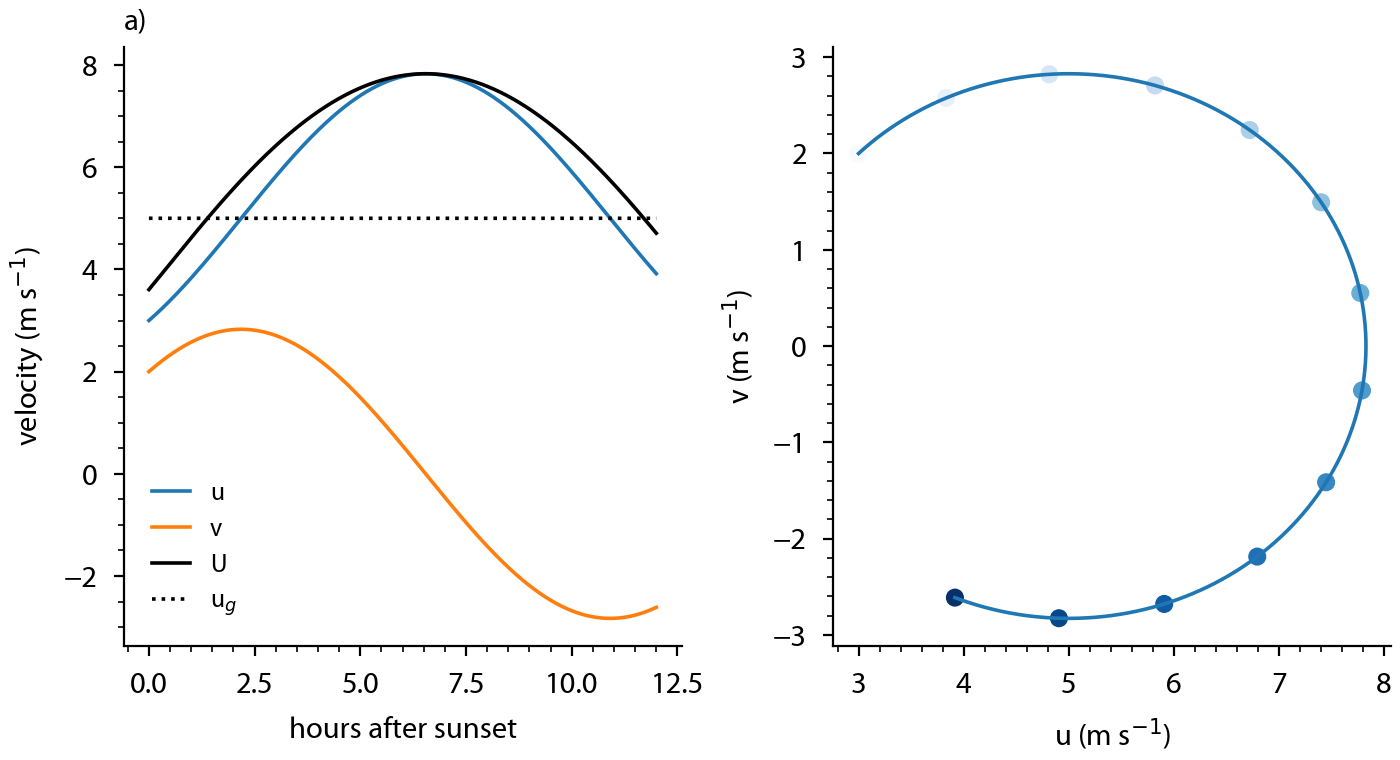
Fig. 14.1 Time evolution of zonal and meridional wind in a decoupled residual layer. Figure a) shows time series, b) shows a scatter plot of the two wind component. Each dot corresponds to an hour with later hours having a darker shade of blue.

14.2. Surface-layer similarity under the influence of stability.

Although we learned about surface layer similarity for a neutral surface layer, in reality, the surface layer is mostly non neutral. We can define a special form of the Richardson number that assumes that fluxes are approximately constant in the surface layer. Note that in this form, we assume that the wind is aligned such that there is only a \(u\)-component and no \(v\).

\[ Ri_\mathrm{f} = \dfrac{\dfrac{g}{\overline{\theta}_\mathrm{v}} \overline{ w^\prime \theta_\mathrm{v}^\prime}} {\overline{u^\prime w^\prime} \pd{\ubar}{z}} = \dfrac{\dfrac{g}{\overline{\theta}_\mathrm{v}} \overline{ w^\prime \theta_\mathrm{v}^\prime}} {- u_*^2 \dfrac{u_*}{\kappa z}} = - \dfrac{ \kappa z \dfrac{g}{\overline{\theta}_\mathrm{v}} \overline{ w^\prime \theta_\mathrm{v}^\prime}} {u_*^3} = \dfrac{z}{L} \]

where \(L\) is the famous Obukhov length

Obukhov length

\[ L \equiv - \dfrac{u_*^3}{\kappa \dfrac{g}{\overline{\theta}_\mathrm{v}} \overline{ w^\prime \theta_\mathrm{v}^\prime}} \]

The Obukhov length \(L\) is the height above the surface where the buoyancy and shear contribution to the TKE evolution are equal in magnitude.

Obukhov discovered that one can write the dimensionless wind gradient \(\phi_m\) as

\[ \dfrac{\kappa z}{u_*} \pd{\ubar}{z} = \phi_m \left( \dfrac{z}{L} \right) \]

and that the value of \(\phi_m\) under neutral conditions is unity. Similarly, we can compute the dimensionless gradient \(\phi_h\) of potential temperature, where we use \(\theta_* = - \overline{w^\prime \theta^\prime} / u_*\), and for which the value is also unity under neutral conditions.

\[\begin{split} \dfrac{\kappa z}{\theta_*} \pd{\overline{\theta}}{z} &= \phi_h \left( \dfrac{z}{L} \right) \\ - \dfrac{\kappa z u_*}{\overline{w^\prime \theta^\prime}} \pd{\overline{\theta}}{z} &= \phi_h \left( \dfrac{z}{L} \right) \end{split}\]

There are many empirical studies around where the functions \(\phi_m\) and \(\phi_h\) are fitted to data. Some examples fitted functions for \(\phi_m\) are

\[ \phi_m \left( \dfrac{z}{L} \right) = 1 + 4.8 \dfrac{z}{L} \]

for stable conditions, and

\[ \phi_m \left( \dfrac{z}{L} \right) = \left( 1 - 19.3 \dfrac{z}{L} \right)^{-\frac{1}{4}} \]

for unstable conditions.

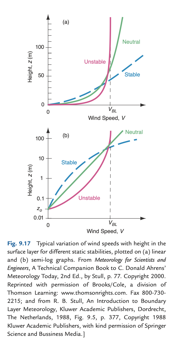
The figure below from Wallace and Hobbs shows how the logarithmic profile is altered by stability.