22. Exercises week 6

\(\def\pafg#1#2{\dfrac{\partial #1}{\partial #2}}\) \(\def\afg#1#2{\dfrac{{\rm d} #1}{{\rm d} #2}}\) \(\def\gemafg#1#2{\pafg{\overline{#1}}{#2}}\)

22.1.

The flux-gradient relationships for momentum and heat (\(\Phi_M\) and \(\Phi_H\)) are related to the exchange coefficients (\(K_M\) and \(K_H\)).

a) Using the first-order closure assumption to parameterize the fluxes and surface layer similarity, show that \(\frac{K_M}{K_H}=\frac{\Phi_H\left(\frac{z}{L}\right)}{\Phi_M\left(\frac{z}{L}\right)}\)

Answer

\[ \overline{w'\theta'} = -K_H \gemafg{\theta}{z} \]

but also

\[\begin{split} \Phi_H &= \frac{\kappa\,z}{\theta_*}\gemafg{\theta}{z} \\ \theta_* &= - \frac{\overline{w'\theta'}}{u_*}\\ \Phi_H &= - \frac{\kappa\,z\,u_*}{\overline{w'\theta'}}\gemafg{\theta}{z} \\ \overline{w'\theta'} &= - \frac{\kappa\,z\,u_*}{\Phi_H \left(\frac{z}{L}\right)}\gemafg{\theta}{z} \end{split}\]

Therefore,

\[\begin{split} -K_H \gemafg{\theta}{z} &= - \frac{\kappa\,z\,u_*}{\Phi_H \left(\frac{z}{L}\right)}\gemafg{\theta}{z} \\ K_H &= \frac{\kappa\,z\,u_*}{\Phi_H \left(\frac{z}{L}\right)} \end{split}\]

Likewise, \(K_M = \frac{\kappa\,z\,u_*}{\Phi_M \left(\frac{z}{L}\right)}\).

\(\Phi_{H,M}\) are basically functions that are devised to introduce the effect of buoyancy on the exchange coefficient. The relationships between \(K_{H,M}\) and \(\Phi_{H,M}\) result in \(\frac{K_M}{K_H}=\frac{\Phi_H\left(\frac{z}{L}\right)}{\Phi_M\left(\frac{z}{L}\right)}\)

b) The moisture flux can be written as

\[ \overline{w'q'}~=~-K_q \pafg{\overline{q}}{z} \]

Knowing that \(\Phi_Q~=~\frac{\kappa z}{q_*} \pafg{\overline{q}}{z}\), show that \(K_Q = \frac{\kappa\,z\,u_*}{\Phi_Q \left(\frac{z}{L}\right)}\)

Answer

Similar to (a),

\[ \overline{w'q'} = -K_Q \gemafg{q}{z} \]

but also

\[\begin{split} \Phi_Q &= \frac{\kappa\,z}{q_*}\gemafg{q}{z} \\ q_* &= - \frac{\overline{w'q'}}{u_*}\\ \Phi_Q &= - \frac{\kappa\,z\,u_*}{\overline{w'q'}}\gemafg{q}{z} \\ \overline{w'q'} &= - \frac{\kappa\,z\,u_*}{\Phi_Q \left(\frac{z}{L}\right)}\gemafg{q}{z} \end{split}\]

Therefore,

\[ -K_Q \gemafg{q}{z} = - \frac{\kappa\,z\,u_*}{\Phi_Q \left(\frac{z}{L}\right)}\gemafg{q}{z} \]

\(K_Q = \frac{\kappa\,z\,u_*}{\Phi_Q \left(\frac{z}{L}\right)}\)

c) For an unstable surface layer, the flux-gradient relationship for \(q\) is

\[ \Phi_Q~=~\left (1-16\frac{z}{L}\right)^{-\frac{1}{2}} \]

Calculate the exchange coefficient at z=300 cm and for a Monin-Obukhov length scale equal to -1.5 m. Calculate the exchange coefficient at the same height but now under neutral conditions. Discuss the results in terms of mixing-length theory.

(\(u_*=0.3~m/s,\kappa=0.4\))

Answer

For this value of \(\frac{z}{L}\) (-1.5), \(\Phi_Q =0.2\), so \(K_Q=1.8\rm\,m^2\,s^{-1}\).

In case of neutral conditions, \(\Phi_Q=1\), so \(K_Q=0.36\rm\,m^2\,s^{-1}\).

In case of a neutral flow, the eddies are smaller. Since the exchange coefficient is a measure of the length scale times a velocity scale (\(K = \cal L \cdot U\)), the exchange coefficient becomes less as well and surface exchange is limited.

22.2.

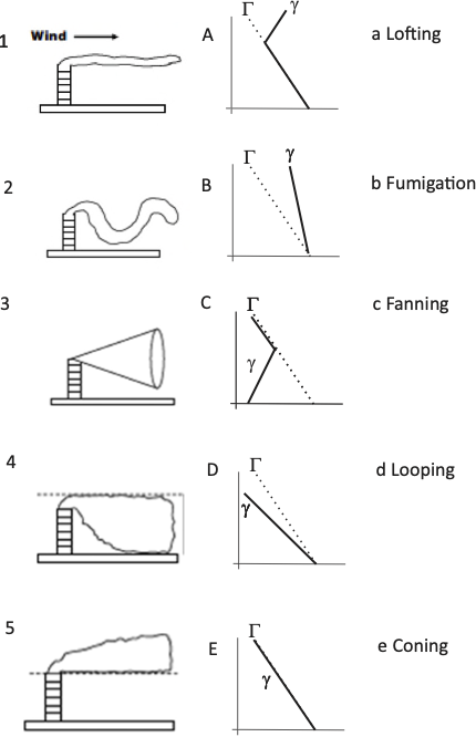
The following picture shows some examples of characteristic shapes of plumes dispersing in various atmospheric regimes.

Link each of the plume shapes with the corresponding name and with the most adequate temperature profile (where the dashed line is the adiabatic lapse rate and the continuous line is the ambient temperature).

Hint

Please focus on matching the plumes (1 to 5) with the profiles (A to E). The names are included for completeness.

Answer

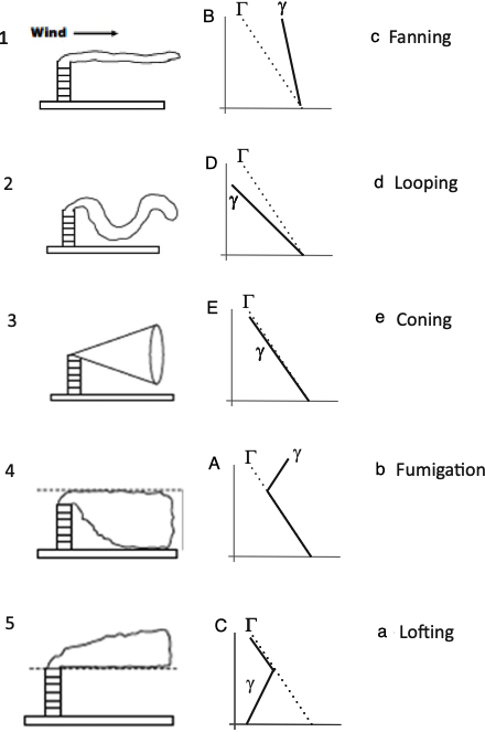
Fig. 22.1 Relation between atmospheric stability and plume dispersion

22.3.

Assuming that the radiative divergence and the phase changes are neglectable, the equation for potential temperature reads

\[ \pafg{\theta}{t}+{u_j}\pafg{\theta}{x_j}~=~\nu_{\theta}\pafg{^2\theta}{x_j^2} \]

a) Derive from this equation that governing equation of the potential temperature fluctuations \(\overline{\theta'^{~2}}\) is

(22.7)\[ \underbrace{\gemafg{\theta'^2}{t}}_{\rm Tendency}+ \underbrace{\overline{u_j}\gemafg{\theta'^2}{x_j}}_{\rm Advection}+\underbrace{2\overline{u_j'\theta'}\gemafg{\theta}{x_j}}_{\rm Production} + \underbrace{\gemafg{{u_j'}\theta'^2}{x_j}}_{Turbulent\ transport} = \underbrace{- 2 \epsilon_\theta}_{\rm Dissipation} \]

Hint

Please note the similarity between this derivation and the derivation of the equation for \(\gemafg{u'^2}{t}\), which gave us the tke equation.

Answer

Question: Governing equation for the potential temperature variance, \(\gemafg{\theta'^2}{t}\)

Known: \(\pafg{\theta}{t}+u_j\pafg{\theta}{x_j}=\nu_\theta \pafg{^2 \theta}{x_j^2}\)

(22.2)\[ \gemafg\theta t + \pafg{\theta'}{t}+\overline{u_j}\gemafg{\theta}{x_j} + \overline{u_j}\pafg{\theta'}{x_j}+{u_j'}\gemafg{\theta}{x_j} + {u_j'}\pafg{\theta'}{x_j} = \nu_\theta \pafg{^2 \overline{\theta}}{x_j^2} + \nu_\theta \pafg{^2 \theta'}{x_j^2} \]

Reynolds averaging Equation (22.2) leads to

(22.3)\[ \gemafg\theta t +\overline{u_j}\gemafg{\theta}{x_j} + \overline{{u_j'}\pafg{\theta'}{x_j}} = \nu_\theta \pafg{^2 \overline{\theta}}{x_j^2} \]

Subtracting Equation (22.3) from Equation (22.2) yields

\[ \pafg{\theta'}{t}+ \overline{u_j}\pafg{\theta'}{x_j}+{u_j'}\gemafg{\theta}{x_j} + {u_j'}\pafg{\theta'}{x_j} - \overline{{u_j'}\pafg{\theta'}{x_j}} = \nu_\theta \pafg{^2 \theta'}{x_j^2} \]

This is multiplied by \(2\theta'\). Combined with the knowledge that \(2x{\rm d}x={\rm d}x^2\), the resulting equation is

\[\begin{split} \pafg{\theta'^2}{t}+ \overline{u_j}\pafg{\theta'^2}{x_j}+2{u_j'\theta'}\gemafg{\theta}{x_j} + {u_j'}\pafg{\theta'^2}{x_j} - 2\theta'\overline{{u_j'}\pafg{\theta'}{x_j}} &= 2\theta'\nu_\theta \pafg{^2 \theta'}{x_j^2} \\ \overline{\pafg{\theta'^2}{t}+ \overline{u_j}\pafg{\theta'^2}{x_j}+2{u_j'\theta'}\gemafg{\theta}{x_j} + {u_j'}\pafg{\theta'^2}{x_j} - 2\theta'\overline{{u_j'}\pafg{\theta'}{x_j}}} &= \overline{2\theta'\nu_\theta \pafg{^2 \theta'}{x_j^2}} \end{split}\]

(22.4)\[ \gemafg{\theta'^2}{t}+ \overline{u_j}\gemafg{\theta'^2}{x_j}+2\overline{u_j'\theta'}\gemafg{\theta}{x_j} + \overline{{u_j'}\pafg{\theta'^2}{x_j}} = 2\nu_\theta \overline{\theta' \pafg{^2 \theta'}{x_j^2} } \]

The last term, \(2\nu_\theta \overline{\theta' \pafg{^2 \theta'}{x_j^2} }\), can be rewritten, similar to the equations of \(u'^2\). To do this, it should be expressed as a function of \(\pafg{\theta'}{x_j}\) and \(\pafg{^2\theta'^2}{x_j^2}\). To tackle this, take a look at the \(2^{\rm nd}\) derivative of \(\theta'^2\). This results in

\[\begin{split} \pafg{^2\theta'^2}{x_j^2} &= \pafg{}{x_j}\pafg{\theta'^2}{x_j}\\ &= \pafg{}{x_j}\left(2\theta'\pafg{\theta'}{x_j}\right) \\ &= 2 \left(\pafg{\theta'}{x_j}\right)^2 + 2 \theta' \pafg{^2\theta'}{x_j^2} \end{split}\]

Rearranging shows that

\[ 2 \theta' \pafg{^2\theta'}{x_j^2} = \pafg{^2\theta'^2}{x_j^2} - 2 \left(\pafg{\theta'}{x_j}\right)^2 \]

Since \(\left|\pafg{^2\theta'^2}{x_j^2}\right|\ll \left|2 \theta' \pafg{^2\theta'}{x_j^2}\right|\) and \(\epsilon_\theta =\nu_\theta\left(\pafg{\theta'}{x_j}\right)^2\), this shows that

(22.5)\[ 2 \nu_\theta \theta' \pafg{^2\theta'}{x_j^2} = - 2 \epsilon_\theta \]

Another term of Equation (22.4) that can be rewritten is \({u_j'}\pafg{\theta'^2}{x_j}\). Since \(\pafg{u_j'}{x_j}=0\) due to incompressibility of the flow,

(22.6)\[\begin{split} {u_j'}\pafg{\theta'^2}{x_j} &= \pafg{u_j'\theta'^2}{x_j} - \theta'^2 \pafg{u_j'}{x_j}\\ {u_j'}\pafg{\theta'^2}{x_j} &= \pafg{u_j'\theta'^2}{x_j} \end{split}\]

Combining Equations (22.4), (22.5) and (22.6) yields

(22.7)\[ \underbrace{\gemafg{\theta'^2}{t}}_{\rm Tendency}+ \underbrace{\overline{u_j}\gemafg{\theta'^2}{x_j}}_{\rm Advection}+\underbrace{2\overline{u_j'\theta'}\gemafg{\theta}{x_j}}_{\rm Production} + \underbrace{\gemafg{{u_j'}\theta'^2}{x_j}}_{Turbulent\ transport} = \underbrace{- 2 \epsilon_\theta}_{\rm Dissipation} \]

b) From the general expression, write the simplified equation if one assumes: steady-state, no advection, horizontal homogeneity and the turbulent transport of \(\overline{\theta'^{~2}}\) is neglectable.

Answer

In the case of steady state, the derivatives to \(t\) become zero. If a horizontal homogeneous situation is studied, the derivatives to \(x\) and \(y\) of Reynolds averaged quantities vanish as well. Therefore, Equation (22.7) turns in

\[ \overline{w}\gemafg{\theta'^2}{z}+2\overline{w'\theta'}\gemafg{\theta}{z} + {\gemafg{{w'}\theta'^2}{z}} = - 2 \epsilon_\theta \]

In case of no subsidence, \(\overline{w}=0\). This eliminates the only form of transport by advection, since the case under study is horizontally homogeneous. Therefore,

\[ 2\overline{w'\theta'}\gemafg{\theta}{z} + {\gemafg{{w'}\theta'^2}{z}} = - 2 \epsilon_\theta \]

Generally, \(3^{\rm rd}\)-order moments are small compared to the other terms in the atmospheric boundary layer. This also holds true for the turbulent transport of potential temperature variance, \(\overline{{w'}\theta'^2}\). Using this assumption, the final equation is

(22.8)\[ \overline{w'\theta'}\gemafg{\theta}{z} = - \epsilon_\theta \]

c) By using the similarity theory scaling functions

\[ \Phi_H~=~\frac{\kappa z}{\theta_*} \pafg{\overline{\theta}}{z}~~~~~~~~ \Phi_{\epsilon\theta}~=~\frac{\kappa z}{u_*\theta_*^2} \epsilon_{\theta}, \]

find the dimensionless form of the equation derived in question b. Discuss the result. What is the value of \(\Phi_{\epsilon\theta}\) under neutral conditions?

Answer

The scaling functions can be used by relating the heat flux and potential temperature gradient to the quantities \(u_*\) and \(\theta_*\) (according to atmospheric surface layer scaling).

\[\begin{split} \theta_* &= - \frac{\overline{w'\theta'}}{u_*}\\ \Phi_H &= \frac{\kappa\,z}{\theta_*}\gemafg{\theta}{z} \end{split}\]

Rewriting results in

\[\begin{split} \overline{w'\theta'} &= - u_* \theta_*\\ \gemafg{\theta}{z} &= \frac{\Phi_H\,\theta_*}{\kappa\,z} \end{split}\]

Substituting these relations into Equation (22.8) results in

\[\begin{split} - u_* \theta_* \frac{\Phi_H\,\theta_*}{\kappa\,z} &= - \epsilon_\theta\\ \Phi_H &= \frac{\kappa\,z}{u_*\theta_*^2}\epsilon_\theta \end{split}\]

In the end, \(\Phi_H=\Phi_{\epsilon\theta}\).

The result shows that, under the conditions that are assumed, all heat that is gained by turbulent transport is dissipated by diffusion.

Under neutral conditions, all flux-gradient relationships are equal to 1.

22.4.

Assuming that the potential temperature increases with height, find the potential temperature at the top of a turbulent layer which becomes laminar at a height of 20 m. The wind profile is given by:

\[\begin{split} \overline{u}(z) &= \frac{u_*}{k}ln\left (\frac {z}{z_o}\right)\\ \overline{v}(z) &= 4 \end{split}\]

The friction velocity is 0.45 m s\(^{-1}\), the potential temperature at the height of the roughness length z\(_o\) is 290 K and assume that the average potential temperature is 295 K. (\(\kappa\) = 0.4, g = 9.8 m \(\rm{s^{-2}}\), z\(_o\) = 1 m). For this exercise, use \(Ri_g^{crit} = 0.25\).

Answer

At the height of 20 meters the flow becomes laminar, meaning:

\[ Ri_g (z=20 \ m.)=\frac{\frac{g}{\overline{\theta}}\frac{\partial \overline{\theta}}{\partial z}}{\left(\frac{\partial u}{\partial z}\right) ^2 +\left(\frac{\partial v}{\partial z}\right) ^2} =0.25\equiv Ri_g^{crit} \]

Rearranging the equation above:

(22.9)\[ \frac{\partial \overline{\theta}}{\partial z}= Ri_g^{crit} \frac{\overline{\theta}}{g} \left[\left(\frac{\partial u}{\partial z}\right) ^2 +\left(\frac{\partial v}{\partial z}\right) ^2 \right] \]

We now calculate \(\frac{\partial u}{\partial z}\) and \(\frac{\partial v}{\partial z}\):

\[\begin{split} \frac{\partial u}{\partial z} &= \frac{u_*}{\kappa}\frac{\partial (ln \frac{z}{z_0})}{\partial z} = \frac{u_*}{\kappa}\frac{1}{z}\\ \frac{\partial v}{\partial z} &= 0 \end{split}\]

Introducing this in Eq. (22.9) we obtain:

\[ \frac{\partial \overline{\theta}}{\partial z}= Ri_g^{crit} \frac{\overline{\theta}}{g} \frac{u_*^2}{\kappa^2}\frac{1}{z^2} \]

We now rearrange and integrate on both sides:

\[ \int_{\theta(z_0)}^{\theta(z)}\partial \overline{\theta}=\int_{z=z_0}^{z}Ri_g^{crit} \frac{\overline{\theta}}{g} \frac{u_*^2}{\kappa^2}\frac{1}{z^2}\partial z \]

Integrating first and then rearranging the terms yields:

\[ \overline{\theta}(z)=\overline{\theta}(z_0) + Ri_g^{crit} \frac{\overline{\theta}}{g} \frac{u_*^2}{\kappa^2} \left( \frac{1}{z_0}-\frac{1}{z}\right) \]

Substituting \(u_*=0.45\), \(\overline{\theta}=295 \ \rm K\), \(\overline{\theta}(z_0)=290 \ \rm K\), \(\kappa=0.4\), \(g=9.8\ \rm{m\ s^{-2}}\), \(z_0=1 \ \rm m\), \(z=20 \ \rm m\), and \(Ri_g^{crit}=0.25\) we obtain

\[ \overline{\theta}(z=20 m)= 299.05 \ \rm K \]

22.5.

The frequency of vertical oscillations for an atmospheric flow is given by the Brunt-Väisälä frequency

\[ N^2=\frac{g}{\overline{\theta_v}} \pafg{\overline{\theta_v}}{z}~~~(s^{-2}) \]

The Brunt-Väisälä frequency is the frequency with which an air parcel oscillates if it’s displaced in a statically stable environment (\(\gemafg{\theta_v}{z} > 0\)).

a) Show that the velocity gradient can be expressed as a function of the gradient Richardson Number and the Brunt-Väisälä frequency as \(\gemafg{u}{z} = \frac{N}{\sqrt{{\rm Ri}_g}}\). Assume that \(\overline{v}(z)=0\).

Answer

Rewrite velocity gradient such that you get \(\gemafg{u}{z}\left({Ri},N\right)\). It’s given that

(22.10)\[ \overline{v}=0 \]

(22.11)\[ N^2=\frac{g}{\overline{\theta_v}} \gemafg{\theta_v}{z} \]

(22.12)\[ {\rm Ri}_g = \frac{\frac{g}{\overline{\theta_v}}\gemafg{\theta_v}{z}}{\left(\gemafg{u}{z}\right)^2+\left(\gemafg{v}{z}\right)^2} \]

Substituting equations (22.10) and (22.11) in Equation (22.12), results in

\[\begin{split} {\rm Ri}_g &= \frac{N^2}{\left(\gemafg{u}{z}\right)^2}\\ \left|\gemafg{u}{z}\right| &= \sqrt{\frac{N^2}{{\rm Ri}_g}} \end{split}\]

As depicted in Fig. 19.2, \(\gemafg{u}{z} > 0\). Since \(N\) is real number, \(N^2 >0\). Also \({\rm Ri}_g > 0\), since we are in a situation with a statically stable atmosphere, which is where \(\gemafg{\theta_v}{z} > 0\). Taking these signs into account, results in: \(\gemafg{u}{z} = \frac{N}{\sqrt{{\rm Ri}_g}}\)

b) Find the velocity at z=30 m for \(N=0.05~s^{-1}\) and Ri=0.2. The surface velocity is 0.

Answer

Since \(N\) and \({\rm Ri}_g\) are given as constants, also \(\gemafg{u}{z}\) is constant. Therefore,

\[\begin{split} \overline{u}\left({z}\right)&=\overline{u}\left({\rm 0\, m}\right)+ z \gemafg{u}{z} ,\\ \overline{u}\left({z}\right)&=0+ z \frac{N}{\sqrt{{\rm Ri}_g}} . \end{split}\]

So, \(\overline{u}\left(30\rm\,m\right)=3.35\rm\,m\,s^{-1}\).

22.6.

Using the following definitions of \(\Phi_M\) and the temperature scaling parameters

\[\begin{split} \Phi_M~=~\frac{\kappa z}{u_*}\pafg{\overline{u}}{z} \\ \theta_*~=~-~\frac{\overline{w'\theta'}}{u_*} \\ \Phi_H~=~\frac{\kappa z}{\theta_*}\pafg{\overline{\theta}}{z} \end{split}\]

a) and assuming that \(\overline{V(z)}=0\), find a relation between the gradient Richardson number and \(z/L\), \(\Phi_M\) and \(\Phi_H\).

Answer

Find \({\rm Ri}_g\left(\frac{z}{L},\Phi_m,\Phi_h\right)\).

We know

\[\begin{split} \theta_* &= -\frac{\overline{w'\theta'}_0}{u_*} \\ \Phi_h &= \frac{\kappa\,z}{\theta_*}\gemafg{\theta}{z} \\ \Phi_m &= \frac{\kappa \, z}{u_*} \gemafg{u}{z}\\ {\rm Ri}_g &= \frac{\frac{g}{\theta_v}\gemafg{\theta_v}{z}}{\left(\gemafg{u}z\right)^2+\left(\gemafg vz\right)^2} \end{split}\]

Using \(\overline{v}=0\), it holds that

\[ {\rm Ri}_g = \frac{\frac{g}{\theta_v}\gemafg{\theta_v}{z}}{\left(\gemafg{u}z\right)^2} \]

\(\gemafg{\theta_v}z\) can be rewritten to \(\gemafg{\theta_v}z = \Phi_h \frac{\theta_*}{\kappa\,z} = \Phi_h \frac{-\overline{w'\theta_v'}_0}{\kappa\,z\,u_*}\) and \(\gemafg uz = \Phi_m\frac{u_*}{\kappa\,z}\). This results in

\[\begin{split} {\rm Ri}_g &= \frac{\frac{g}{\theta_v}\Phi_h \frac{-\overline{w'\theta_v'}_0}{\kappa\,z\,u_*}}{\left(\Phi_m\frac{u_*}{\kappa\,z}\right)^2} \\ &= - \frac{\Phi_h}{\Phi_m^2} \frac{g\,\overline{w'\theta_v'}_0\,\kappa\,z}{\overline{\theta_v}\,u_*^3} \\ &= - \frac{\Phi_h}{\Phi_m^2} \frac{\kappa\,g\,\overline{w'\theta_v'}_0}{u_*^3\,\overline{\theta_v}} z \end{split}\]

Since

\[ L = - \frac{u_*^3\,\overline{\theta_v}}{\kappa\,g\,\overline{w'\theta_v'}_0} \]

the final result is \({\rm Ri}_g=\frac{\Phi_h}{\Phi_m^2}\frac{z}{L}\)

b) Under very stable conditions \(\Phi_M~=~ \alpha_M\frac{z}{L}\) and \(\Phi_H~=~ \alpha_H\frac{z}{L}\) where (\(\alpha_M=\alpha_H \approx 5\)). Discuss the value of the Richardson number under this condition.

Hint

Typical stability functions are

\[\begin{split} \Phi_m &= 1 +\left(\frac{4.7z}{L}\right)\\ \Phi_h &= \frac{K_M}{K_H} +\left(\frac{4.7z}{L}\right) \end{split}\]

For very stable conditions, \(\frac{z}{L}\gg 1\), so \(\Phi_m \approx \Phi_h\) with a value of \(4.7\frac{z}{L}\).

Answer

Under these very stable conditions, substituting the \(\Phi\)-functions, it can be seen that \({\rm Ri}_g = \frac{\alpha_h\frac{z}{L}}{\left(\alpha_m\frac{z}{L}\right)^2}\frac{z}{L} = \frac{\alpha_h}{\alpha_m^2}\approx \frac{1}{5}=0.2\).

This Richardson gradient number is independent on height. However, note that for this Richardson number, the flow should become turbulent. The problem in the assumed limit is that the \(\Phi\)-functions are usually evaluated in a range of about \(-2<\frac{z}{L}<2\). When taking the limit to very high or very low \(\frac{z}{L}\), the functions are not valid anymore.

22.7.

In a fertilized field a constant flux of nitric oxide (\(NO\)) has been measured (\(\overline{w'NO'}=0.1~ppb~m/s\)) with a concentration of NO at ground level equal to 5 ppb. Additional measurements showed that \((z/L) \approx 0\) and the friction velocity was 0.3 m/s. (\(z_o=10~cm\))

a) Find the concentration of NO at 10 m. Plot the profile of NO(z).

Answer

Find \({\rm NO}\left(z\right)\) and plot it.

Known:

\[\begin{split} \overline{w'{\rm NO}'} &= 0.1\rm\,ppb\,m\,s^{-1}\\ {\rm NO}\left(0\rm\,m\right) &= 5\rm\,ppb\\ \frac{z}{L} &\approx 0 \\ u_* &= 0.3\rm\,m\,s^{-1}\\ z_0 &= 0.1 \rm\,m \end{split}\]

Since \(\frac{z}{L}\approx 0\), we know that \(\Phi_{\rm NO} \approx 1\), so

\[\begin{split} \Phi_{\rm NO} &= \frac{\kappa\,z}{{\rm NO}_*} \gemafg{{\rm NO}}{z}\\ 1 &= \frac{\kappa\,z}{{\rm NO}_*} \gemafg{{\rm NO}}{z} \end{split}\]

Since the definition of \({\rm NO}_*\) (using Monin-Obukhov scaling) is given by

\[ {\rm NO}_* = -\frac{\overline{w'{\rm NO}'}}{u_*} \]

the flux gradient relationship can be rewritten to

\[\begin{split} 1 &= - \frac{\kappa\,z\,u_*}{\overline{w'{\rm NO}'}} \gemafg{{\rm NO}}{z}\\ \gemafg{{\rm NO}}{z} &= -\frac{\overline{w'{\rm NO}'}}{\kappa\,z\,u_*} \\ \int_{z_1}^{z_2}{\gemafg{{\rm NO}}{z}{\rm d}z} &= -\int_{z_1}^{z_2}{\frac{\overline{w'{\rm NO}'}}{\kappa\,z\,u_*}{\rm d}z}\\ \overline{{\rm NO}}\left(z_2\right) -\overline{{\rm NO}}\left(z_1\right) &= -\frac{\overline{w'{\rm NO}'}}{\kappa\,u_*} \int_{z_1}^{z_2}{\frac{1}{z}{\rm d}z} \end{split}\]

considering a constant NO-flux near the surface. Therefore,

(22.13)\[ \overline{{\rm NO}}\left(z_2\right) = \overline{{\rm NO}}\left(z_1\right) - \frac{\overline{w'{\rm NO}'}}{\kappa\,u_*} {\rm ln}\frac{z_2}{z_1} \]

In this case, \(z_1=z_0=0.1\rm\,m\), \({\rm NO}\left(z_1\right)=5\rm\,ppb\) and \(z_2=z\). Therefore, substituting the known variables, \(\overline{\rm NO}\left(z\right)= 5 - \frac{5}{6}{\rm ln}\frac{z}{0.1\rm\,m}\quad\left(\rm ppb\right)\).

The plot of this equation is shown in Fig. 22.2. The concentration at 10 m height is 1.16 ppb.

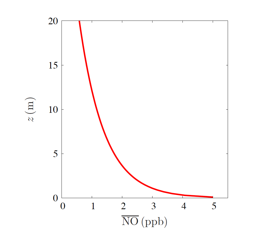
Fig. 22.2 Vertical profile of NO in ppb

b) At which height the NO concentration is lower than \(70\%\) with respect the ground value.

Answer

For which \(z\) is \(\overline{\rm NO}\left(z\right)=0.7\cdot\overline{\rm NO}\left(0\rm\,m\right)\)?

Equation (22.13) shows that in that case

\[\begin{split} \overline{{\rm NO}}\left(z\right) &= \overline{{\rm NO}}\left(z_0\right) - \frac{\overline{w'{\rm NO}'}}{\kappa\,u_*} {\rm ln}\frac{z}{z_0}\\ 0.7\,\overline{{\rm NO}}\left(z_0\right) &= \overline{{\rm NO}}\left(z_0\right) - \frac{\overline{w'{\rm NO}'}}{\kappa\,u_*} {\rm ln}\frac{z}{z_0} \end{split}\]

This results in

\[\begin{split} \frac{\overline{w'{\rm NO}'}}{\kappa\,u_*} {\rm ln}\frac{z}{z_0} &= 0.3\,\overline{{\rm NO}}\left(z_0\right)\\ {\rm ln}\frac{z}{z_0} &= \frac{0.3\,\kappa\,u_*\,\overline{{\rm NO}}\left(z_0\right)}{\overline{w'{\rm NO}'}}\\ z &= z_0\,{\rm e}^\frac{0.3\,\kappa\,u_*\,\overline{{\rm NO}}\left(z_0\right)}{\overline{w'{\rm NO}'}} \end{split}\]

Substituting the values that are given results in \(z=60.5\rm\,cm\)