13. Turbulence spectra#
Questions to be answered in this chapter
What is an energy spectra and how it is derived?
How does a turbulence kinetic energy spectra look?
What is the explanation for the famous \(-5/3\) slope of the turbulence kinetic energy spectra?
13.1. Fourier transform and energy spectrum#
Fourier transforming data allows us to transform data from physical to spectral space. Fourier transformation goes as following
although since we generally work with time series of spatial series with equal sampling interval we use the discrete Fourier transform
By doing so, we can write a time or spatial series as a sum of waves with varying phase and amplitude.
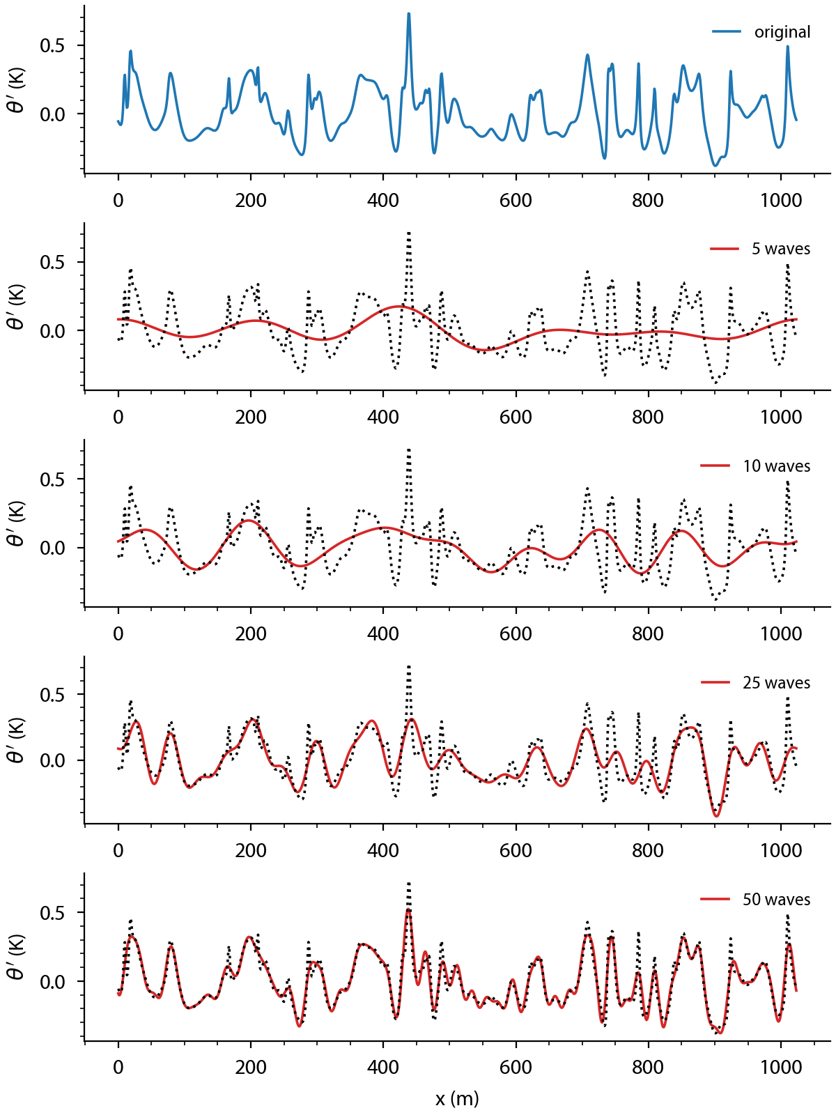
Fig. 13.1 Potential temperature near the surface of the convective boundary layer captures in waves.#
Based on the waves we can calculate its contribution to the variance by taking the square of its absolute value.
13.2. The spectral structure of the inertial subrange of turbulence#
The turbulence kinetic energy \(e\) can be constructed from its spectral energy \(E(k)\) (energy per wave number \(k\)) following
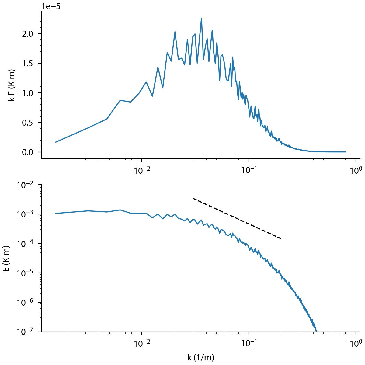
Fig. 13.2 Spectral energy of the potential temperature near the surface of the convective boundary layer.#
If we assume a strict separation between production and dissipation in terms of length and time scales, there must exist a region that only transfers energy from the largest to the smallest scales. We call this region the inertial subrange, and the only parameter relevant there is \(\epsilon\). Note that viscosity \(\nu\) does not play a role here yet.
Following the same dimensional reasoning as before, and noting that only \(\epsilon\) matters, the spectral energy \(E\) must be related to wave number \(k\) and dissipiation \(\epsilon\) as
Kolmogorov scaling of the intertial subrange
The result that the spectral energy \(E\) for a certain wave number is proportional to wave number \(k\) to the power \(-5/3\) is one of the most fundamental properties of high-Reynolds number turbulent flows.