21. Exercises week 5#
\(\def\pafg#1#2{\dfrac{\partial #1}{\partial #2}}\) \(\def\afg#1#2{\dfrac{{\rm d} #1}{{\rm d} #2}}\) \(\def\gemafg#1#2{\pafg{\overline{#1}}{#2}}\)
Hint
Remember that \(H\ =\ \rho\ c_p\ \overline{w'\theta'}\). If no values are given, use \(\rho\ c_p\ = 1231\ J\ K^{-1}\ m^{-3}\).
21.1. #
The following figure shows the raw observation of the wind speed.
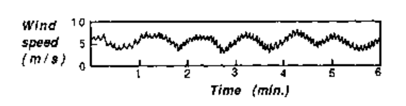
Sketch your best guess of the spectrum of the wind velocity as function of the period (min), the frequency (cycles/min) and the wave-number (cycles/m).
Answer
It should be visible in the figure at which frequencies the eddies contain most energy. In this exercise, not the angular frequencies, \(\left(\omega=\frac{2\pi}{T}\right)\), and wave numbers, \(\left(k=\frac{2\pi}{\lambda}\right)\), are used, but the ordinary ones: \(f=\frac{1}{T}\) and \(\nu=\frac{1}{\lambda}\). In these equations \(T\) and \(\lambda\) denote the corresponding period and length scale. The periods that seem most important are 1 minute and 0.1 minute (6 s). The signal with a time scale of 1 minute contains most energy. The corresponding sketch is shown in Fig. 21.1.
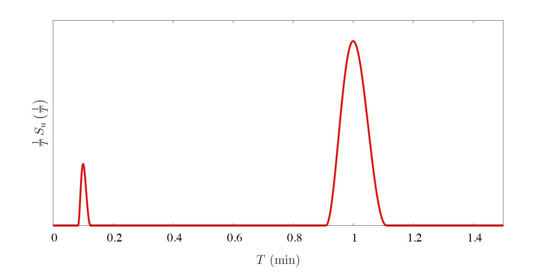
Fig. 21.1 Spectrum of the wind velocity as a function of time.#
The conversion from time period to frequency is straight forward. However, the dependency on the wave number is a bit harder.
Since \(\overline{u} = 5\rm\,m\,s^{-1}\) according to the observations, it is known that \(\nu = \frac{f}{\overline{u}} = f \frac{1}{5\rm\,m\,s^{-1}} = f \frac{1}{300} \rm\frac{min}{m}\). According to Taylor’s frozen turbulence assumption, \(f\) and \(\nu\) are proportional to each other (Equation (21.1)). Therefore, the sketch for these two variables are combined in Fig. 21.2.
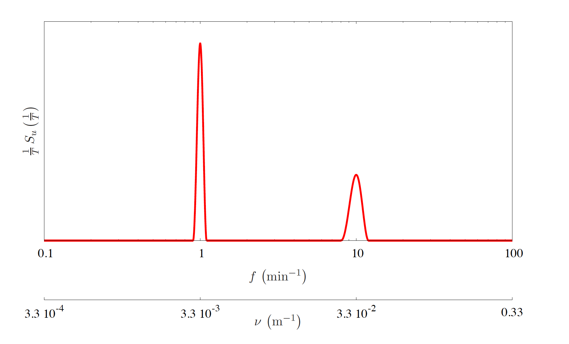
Fig. 21.2 Spectrum of the wind velocity as a function of frequency, \(f\), and wave number, \(\nu\).#
21.2. #
The spectra of the vertical velocity was calculated from sonic measurements taken under convective conditions at Cabauw (23 August 2001 at 12 UTC).
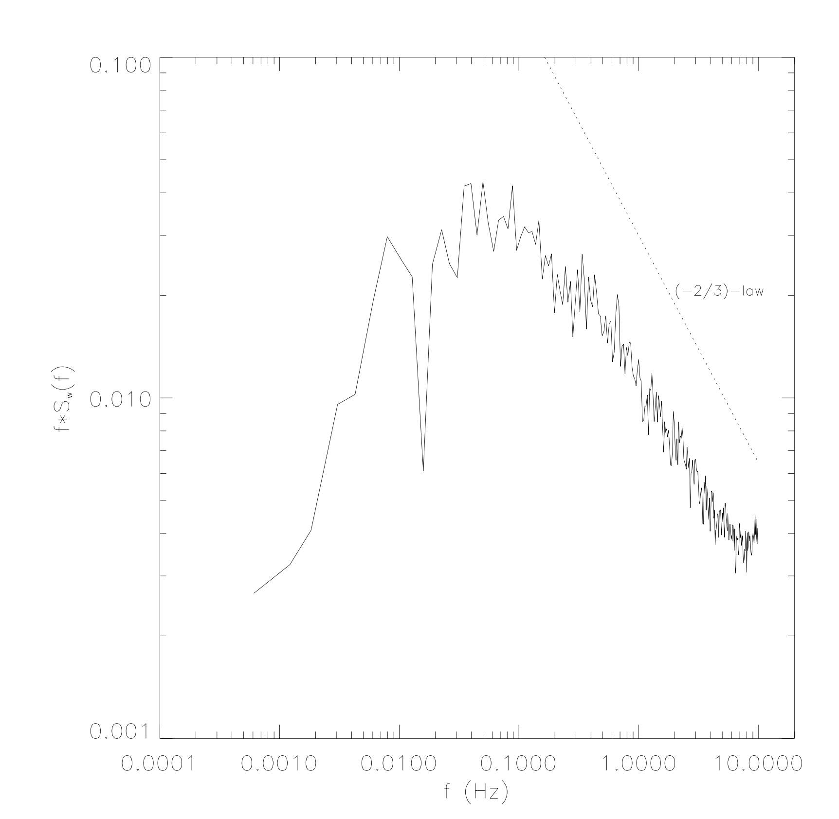
Fig. 21.3 Power spectra of the vertical velocity measured by means of a sonic at 2 m at Cabauw during the 23th August 2001#
a) Describe the different regions in this power spectrum of the vertical velocity
Answer
Energy containing/producing range
Inertial subrange: redistribution, transport processes
Dissipation range
The border between 1 and 2 lies at the beginning of the relative straight decay of turbulence and the border between 2 and 3 at the end of this straight line.
b) Discuss the validity of the Reynolds decomposition for the vertical velocity \(w= \overline{w}~+~w'\)
Hint
It’s often stated that \(\overline{w}=0\), but over how much time should we average, such that this assumption is valid?
Answer
If the spectrum is high, there is still a lot of energy associated with fluctuations of that frequency. It is visible that for \(f>0.005\rm\,Hz\), the energy is still high, so there are many fluctuations of that frequency. To be able to average out all fluctuations for \(\overline{w}\), one should measure long enough.
so \(T_{\rm Av.}>200\rm\,s\).
c) If \(U=5~m/s\), find the characteristic length scale for this convective boundary layer.
Answer
The characteristic length scale is the scale that contains most energy. From the figure, the corresponding frequency, \(f\), is 0.05 Hz.
Therefore, \(\lambda_{\rm char.} = 100\rm\,m\).
d) What is the frequency response of the sonic anemometer.
Answer
Frequency response: the frequency with which is measured. This frequency corresponds to the highest frequency that’s present in the corresponding Fourier spectrum. However, to prevent aliasing, spectra are evaluated until the Nyquist frequency, \(f_{Nyquist}\). Since \(f_{Nyquist} = \frac{f_{max}}{2}\) and \(f_{nyquist}=10\rm\,Hz\), we know that \(f_{max}=20\rm\,Hz\).
e) In the inertial subrange \(S(k) \cong \alpha \epsilon^{\frac{2}{3}} \kappa^{-\frac{5}{3}}\). Using Taylor’s hypothesis of frozen turbulence that relates frequencies and wave numbers with the mean wind (\(f = U K\)), we can derive that in the inertial subrange, the region which separates the energy-containing region from the dissipation region, the density of the energy spectrum follows
where \(\alpha\) is a constant equal to 0.6; \(\epsilon\) is the dissipation of the turbulent kinetic energy and \(f\) is the frequency. Using the values of the figure, calculate the characteristic length scale at the dissipation range which is given by
where \(\nu\) is the kinematic viscosity of air (\(1.5~10^{-5} m^2/s)\). (and \(U=5~m/s\) as in question c)
Answer
Calculate the length scale of dissipation (Kolmogorov length scale): the length scale for which motions are dissipated by molecular processes. This is the lower bound of the length scales that can be evaluated using the governing equations without losing their physical meaning.
\(\nu=1.5\,10^{-5}\rm\,m^2\,s^{-1}\), but \(\epsilon\) has to be calculated. In the inertial subrange
Since \(f=1\rm\,Hz\) lies in this range, we can evaluate this equation for this value and
This is in SI units (\(\rm\,m^2\,s^{-3}\)). Filling it up results in \(\eta = 3.1\cdot\,10^{-3}\rm\,m\), so \(\eta=3.1\rm\,mm\)
f) Calculate the ratio between the characteristic length scale of the boundary layer (question c) and the dissipation length scale (question e). Discuss the result.
Answer
This ratio shows how many times the smallest scale involved has to be resolved in order to also resolve the characteristic process for at least one period. The ratio is \(R=\frac{100\rm\,m}{3\rm\,mm}\), so \(R=3 \cdot 10^4\).
21.3. #
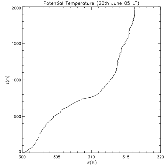
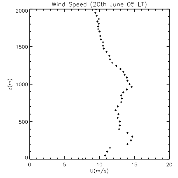
The figures below show the vertical profiles of potential temperature and wind speed observed at the Southern Great Plains in USA during the night of 20th June 1997. By analyzing them we can determine some of the main characteristics of the nocturnal boundary layer.
a) Describe both vertical profiles.
Answer
Temperature profile: This is a stable boundary layer that has a height of approximately 750 m. Above this height, the (slightly less stable) free troposphere is present.
Wind speed profile: A low level jet is present between 200 and 400 m height. Ignoring this jet, the wind speed increases with height until 950 m. Above this height, the wind speed decreases with height.
b) Determine the boundary layer height according the potential temperature profile and the wind speed. Discuss your criteria and the estimation of the height.
Answer
Using the potential temperature gradient, there are multiple criteria possible, resulting in different heights.
In the residual layer \(\pafg{\theta}{z}=0\): This only occurs at the top of the profile
In the residual layer \(\pafg{\theta}{z}\) is small: This is valid at \(h=1000\rm\,m\) and above.
Above the residual layer, there is an inversion where \(\pafg{\theta}{z}\) is large: this occurs around 750m.
For the wind speed, the location of the low level jet is used. The maximum wind speed in this jet is at a height of 250 m.
c) An air parcel in a stable environment will oscillate when displaced vertically. This oscillation can be quantified with the Brunt-Väisälä frequency. By inverting this frequency, one obtains the period of the oscillation of a parcel in a statically stable environment related to the presence of gravity (buoyancy) waves.
Calculate the Brunt-Väisälä frequency (\(N = \sqrt{\frac{g}{\theta_v}\gemafg{\theta_v}{z}}\)) and the oscillation period for an air parcel that is displaced from the surface. Discuss the dependence of this oscillation period as a function of the potential temperature gradient.
Answer
This results in \(N=2.02 \cdot 10^{-2}\rm\,s^{-1}\)
This frequency corresponds to a period of 49.5 s.
The oscillation of an air parcel in a statically stable environment is like a mass that is attached to a spring. In this case, an air parcel that is displaced from its original position experiences a force to return to this position, proportional to the potential temperature gradient. Therefore, in situations characterized by a stronger gradient, the restoring force is larger. This leads to higher accelerations and, consequently, higher frequencies. Therefore, more stable environments should result in faster oscillations, which are quantified by the Brunt-Väisälä frequencies.
d) During the night, the friction velocity and the sensible heat flux were almost constant on time with the values 0.6 \(ms^{-1}\) and -50 \(Wm^{-2}\), respectively. Calculate the flux Richardson number. What is the role of buoyancy and shear in this nocturnal boundary layer?
Answer
Assuming \(\overline{w'\theta_v'}=\overline{w'\theta'}\) and converting the sensible heat flux to kinematic heat flux, results in \(\overline{w'\theta_v'}=-0.0406\rm\,K\,m\,s^{-1}\). Furthermore,
Substituting these values results in \({\rm Ri}_f = 0.074\)
\({\rm Ri}_f\) is larger than 0, but smaller than 1, thus shear production is sufficiently high to counter buoyancy destruction related to statically stable conditions.
21.4. #
These vertical profiles for potential temperature were measured in USA at 00.07 and 04.02 local time during the field experiment CASES-99. Focusing mainly on the sounding observations:
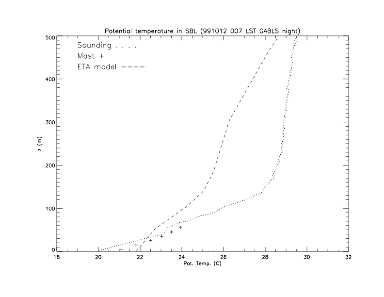
Fig. 21.4 Potential temperature profile at 00.07 LT.#
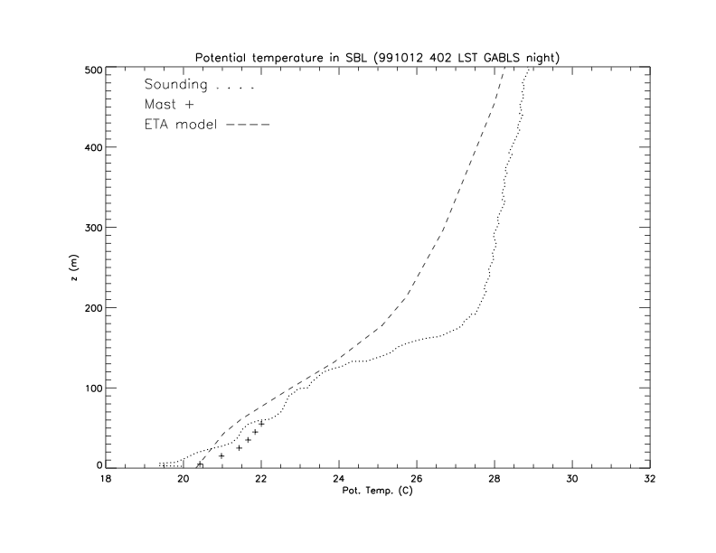
Fig. 21.5 Potential temperature profile at 04.02 LT.#
Describe both profiles of the potential temperature. Estimate the evolution of the boundary layer height and the gradient of the potential temperature from the surface to the top of the boundary layer.
Answer
Both profiles are stable boundary layers.
Fig. 21.4 shows a boundary layer with a height of 140 m. In this layer, the potential temperature gradient, \(\gemafg{\theta}{z}\), is equal to 57 K km\(^{-1}\).
Fig. 21.5 shows a boundary layer with a height of 180 m. In this layer, the potential temperature gradient is equal to 45 K km\(^{-1}\).
The evolution of the boundary layer height is 40 m over 4 hours, so \(\pafg{h}{t}=10\rm\,m\,hr^{-1}\).
The evolution of the gradient of the potential temperature is equal to \(-12\rm\,K\,km^{-1}\) over 4 hours, so \(\pafg{}{t}\gemafg{\theta}{z}=-3\rm\,K\,km^{-1}\,hr^{-1}\)
21.5. #
The one-dimensional equation that governs the heat budget during stable conditions reads
The longwave radiative term \(\frac{1}{\rho c_p}\pafg{Q^*}{z}\) can be calculated using a bulk approach. \(Q^*\) is the the new upward longwave radiative flux. In short, we can define three layers: surface (s), middle (m) and top (t) that are radiatively active according to the Stefan-Boltzmann expression:
where L is the generic expression for the longwave radiative cooling.
Hint
The situation that is described is:

There is upward longwave radiation from the surface to the middle layer and from the middle layer to the top layer and there is downward longwave radiation from the top layer to the middle layer and from the middle layer to the surface.
a) Derive a bulk expression of the longwave radiative divergence (\(\pafg{Q^*}{z}\)) for these three layers.
Answer
The radiative divergence is \(\afg{Q^*_{\rm tot}}{z}\), where \(Q^*_{\rm tot}\) is the net upward longwave radiation. In the case of the bulk expression, assuming finite differences, this becomes
This is evaluated between the two interfaces (the lower is between the surface and the middle layer and the upper is between the middle layer and the top layer). \(\Delta Q^*_{\rm tot}\) is the difference in \(Q^*_{\rm tot}\) between these two interfaces and \(\Delta z\) the height over which this bulk approach is applied. Since \(Q^*\) is defined as upward radiation we can evaluate the values of net \(Q^*\) at the interfaces as
Since \(\Delta\ Q^*_{\rm tot} = Q^*_{\rm interface\,2} - Q^*_{\rm interface\,1}\),
b) Assuming that the emissivity at these layers is equal (\(\epsilon_{IR}=0.78\)) and neglecting the divergence of the turbulent flux term, calculate the tendency term \(\pafg{\overline{\theta}}{t}\). Assume that the potential temperature profile is linear and follows:
You can consider that the surface layer is at z\(_o\) = 0.1 m and \(\theta (z_o)\) = 292 K. The other layers middle and top are at 5 and 10 meters respectively. In consequence, the interfaces are approximately at 2.55 and 7.5 meters.
Hint
Use \(\rho\,c_p=1231\rm\, J\,m^{-3}\ K{-1}\).
Assume (since we are close to the surface) that \( T = \theta \).
Answer

Fig. 21.6 Vertical profiles of \(\theta\) in red for exercise b (linear profile) and in blue for exercise c (logarithmic profile).#
Under these conditions,
The interfaces are located at 2.55 m and 7.5 m, so \(\Delta z = 4.95\ \rm{m}\).
With the linear temperature profile, we find the following temperatures:
\(\rho\,c_p=1231\rm\,\frac{W\,m^{-2}}{K\,m\,s^{-1}}\), \(\sigma_{\rm SB}=5.67\cdot 10^{-8}\rm\,W\,m^{-2}\,K^{-4}\) and \(\epsilon_{\rm IR} = 0.78\), so \(\frac{\epsilon_{\rm IR}\, \sigma_{\rm SB}}{\rho\,c_p} = 3.59\cdot 10^{-11} \rm K^{-3}\,m\,s^{-1}\).
c) Repeat now the calculation but assuming a logarithmic profile for the potential temperature that reads:
with
Use the following values to complete the expression: \(\overline{w'\theta'}\) = - 0.0195 K m s\(^{-1}\), u\(_*\)=0.1 m, z\(_o\)=0.1 m and von Karman constant equal to 0.4. Similar to (b), assume the surface layer at z\(_o\)=0.1 m and \(\theta (z_o)\)=292 K; and layers middle and top at 5 and 10 meters respectively.
Answer
Substituting the variables leads to
The constants are equal to exercise b, so
Note that using the rounded temperatures results in wrong answers. This is due to the power of 4 of the temperature.
d) Discuss your results from a perspective of the tendency of the temperature \(\pafg{\overline{\theta}}{t}\). Based on the results of (b) and (c), discuss the most probable profile observed during stable conditions.
Answer
According to a linear potential temperature profile, the middle layer would actually heat up due to radiation by 0.079 K per hour. This is in contradiction with the knowledge that at night radiative cooling takes effect.
The more realistic logarithmic profile results in a cooling effect due to radiation by 4.1 K per hour. This is more reasonable.
In conclusion, the nocturnal temperature profile that is most probable to be observed is the logarithmic profile.
21.6. #
The momentum equation for the \(\overline{u}\) and \(\overline{v}\)-component during diurnal and nocturnal conditions reads:
where \(u_g\) is the geostrophic wind in the u direction and f is the Coriolis parameter. We assume that \(v_g\)=0.
a) Derive expressions for \(\overline{u}\) and \(\overline{v}\) during day conditions. In diurnal conditions, one can assume that the wind is in steady-state.
Answer
Since we are evaluating (diurnal) stationary conditions,
Therefore,
b) Calculate the \(\overline{u}\) and \(\overline{v}\)-components during the night. To this end, take the following steps:
Under nocturnal conditions, the friction suddenly disappears above the surface layer. Discuss the validity of this assumption. Use this assumption to simplify the momentum equations.
Answer
Under nocturnal conditions, the flow can become laminar. As a result, the different layers in the flow can decouple from each other and the surface. This lowers friction and, therefore, shear and the momentum flux in the \(z\)-direction. In consequence, the wind accelerates. Therefore, finally the shear decreases in total a little, but the momentum flux decreases to a very low value. Therefore, it can be neglected with respect to the Coriolis and horizontal pressure gradient terms.
(21.5)#\[ \gemafg{u}{t} =f\,\overline{v} \](21.6)#\[ \gemafg{v}{t} =f\,\left(u_g-\overline{u}\right) \]Derive a second-order differential equation for the \(\overline{u}-u_g\) component
Answer
Considering that \(u_g\) is a constant,
\[\begin{split} \gemafg{u}{t} &= \gemafg{u}{t}-\gemafg{u_g}{t}\\ &= \pafg{\left(\overline{u}-u_g\right)}{t} \end{split}\]Combined with Equations (21.5) and (21.6), this results in
\[\begin{split} {\pafg{^2\left(\overline{u}-u_g\right)}{t^2}} &= \pafg{}{t}\pafg{\overline{u}}{t} \\ &= \pafg{}{t}\left(f\,\overline{v}\right)\\ &= f\,\gemafg{v}{t}\\ &= f^2\,\left(u_g-\overline{u}\right)\\ {\pafg{^2\left(\overline{u}-u_g\right)}{t^2}} &= - f^2\,\left(\overline{u}-u_g\right) \end{split}\]The expression found for \(\overline{u}-u_g\), corresponds to a harmonic oscillator equation, \(\pafg{^2 x}{t^2}=-k\,x\).
In this case \(x\) is equal to \(\left(\overline{u}-u_g\right)\) and \(k=f^2\).
A general solution is \(x=A\sin\left(\sqrt{k}t\right)+B\cos\left(\sqrt{k}t\right)\).
Hint
We can prove that the solution
\[ \overline{u}-u_g=A sin(ft) + B cos (ft) \]is a correct solution:
\[\begin{split} \pafg{^2 x}{t^2} &= \pafg{^2}{t^2}\left(A\sin\left(\sqrt{k}t\right)+B\cos\left(\sqrt{k}t\right)\right) \\ &= \pafg{^2 A\sin\left(\sqrt{k}t\right)}{t^2} + \pafg{^2 B\cos\left(\sqrt{k}t\right)}{t^2}\\ &= A \pafg{\sqrt{k} \cos\left(\sqrt{k}t\right)}{t} - B \pafg{\sqrt{k} \sin\left(\sqrt{k}t\right)}{t} \\ &= A \sqrt{k} \left(-\sqrt{k}\sin\left(\sqrt{k}t\right)\right) - B \sqrt{k} \left(\sqrt{k}\cos\left(\sqrt{k}t\right)\right) \\ &= - k \left(A\sin\left(\sqrt{k}t\right)+B\cos\left(\sqrt{k}t\right)\right)\\ &= -k \, x \end{split}\]Now use the general solution for the harmonic oscillator and the following initial conditions to find an expression for \(\overline{u}\) and \(\overline{v}\):
\[ \overline{u}(t=0) = u_g-F_{v}(t=0) \]\[ \overline{v}(t=0) = F_{u}(t=0) \]where \(F_{u}(t=0) = \frac{1}{f} \pafg{\overline{w'u'}}{z}\) and \(F_{v}(t=0) = \frac{1}{f}\pafg{\overline{w'v'}}{z}\).
Note that these initial conditions are the daytime steady-state conditions that were derived in question a.
Answer
\(\overline{u}-u_g = A\sin\left(ft\right)+B\cos\left(ft\right)\), so
\[\begin{split} \overline{u}(0) &= u_g + B\\ &= u_g - F_v(0)\\ B &= -F_v(0)\\ \overline{u} &= u_g + A\sin\left(ft\right)- F_v(0) \, \cos\left(ft\right) \end{split}\]Since \(\overline{v} = \frac{1}{f}\gemafg{u}{t}\),
\[\begin{split} \overline{v} &= \frac{1}{f}\left(A f\cos\left(ft\right) + F_v(0) f \sin\left(ft\right) \right) \\ &= A \cos\left(ft\right) + F_v(0) \sin\left(ft\right) \end{split}\]Using, the second boundary condition,
\[\begin{split} \overline{v}(0) &= A \\&= F_u(0)\\ A &= F_u(0) \end{split}\]All in all, the equations for \(\overline{u}\) and \(\overline{v}\) are
\[\begin{split} \overline{u} &= u_g + F_u(0) \sin\left(ft\right) - F_v(0) \cos\left(ft\right)\\ \overline{v} &= F_v(0) \sin\left(ft\right) + F_u(0) \cos\left(ft\right) \end{split}\]This can be written as
\[\begin{split} \overline{u} &= u_g + \frac{1}{f} \gemafg{w'u'}{z} \sin\left(ft\right) - \frac{1}{f} \gemafg{w'v'}{z} \cos\left(ft\right)\\ \overline{v} &= \frac{1}{f} \gemafg{w'v'}{z} \sin\left(ft\right) + \frac{1}{f} \gemafg{w'u'}{z} \cos\left(ft\right) \end{split}\]
c) Plot the \(\overline{u}\) and \(\overline{v}\)-components for a full period T=2\(\pi\)/f, using the following values:
f = 10\(^{-4}\) s\(^{-1}\), F\(_{u}(t=0)\) = F\(_{v}(t=0)\) = 3 m s\(^{-1}\), \(u_g\) = 10 m s\(^{-1}\), and \(v_g\) = 0 m s\(^{-1}\).
Answer
The wind velocities, \(\overline{u}\) and \(\overline{v}\) are plotted in Fig. 21.7.
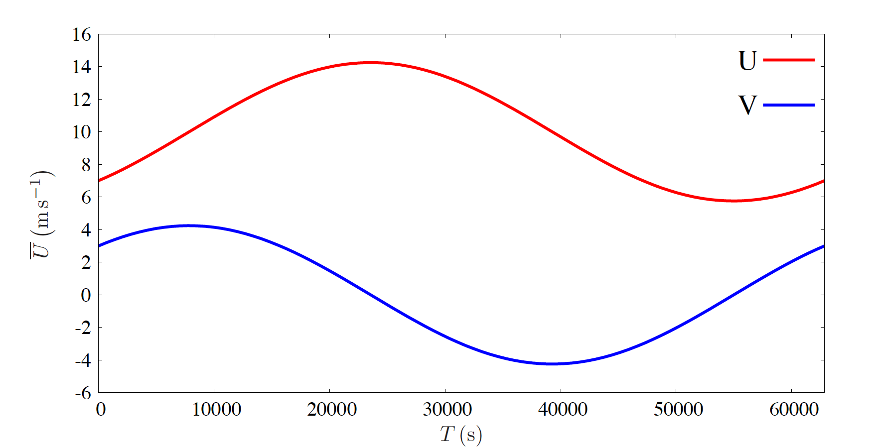
Fig. 21.7 Evolution of wind velocities.#
d) Derive an expresion for \(\left(\overline{u}-u_g\right)^2 + \overline{v}^2\). Use this expression to explain how the wind changes over time.
Answer
Realize that
Therefore,
Combining these 2 equations results in
Since the right-hand side is a constant, this equation states that \(\left(\overline{u},\overline{v}\right)\) progresses in time as a circular movement around \(\left(u_g,0\right)\) at a distance of \(\sqrt{F_u^2(0) + F_v^2(0)} = 3\sqrt{2}\rm\,m\,s^{-1}\)
This can also be seen from Fig. 21.7.
21.7. #
The conservation equation for the potential temperature in a Stable Boundary Layer reads (neglecting phase changes)
a)By using a bulk approach, calculate the divergence of the net upward longwave radiation (\(Q^*=F_{up}-F_{down}\)). Remember that the longwave radiation follows the Stefan-Boltzmann law:
The following values in the three-layer model of the stable boundary layer are suggested. At the surface, \(T_s=290~K\) and \(\epsilon_s=0.78\).
In the layer that represents the SBL, \(T_m=296~K\) and \(\epsilon_m=0.78\).
Finally, at the top of the SBL \(T_t=298~K\) and \(\epsilon_t=0.78\).
The boundary layer height is equal to 25 m. Additional data to calculate the divergence of the net longwave radiation are: \(\rho\ =\ 1.2261\ Kg\ m^{-3}\), \(c_p\ =\ 1004\ J\ Kg^{-1}\ K^{-1}\).
Answer
The term that is asked for is \(\pafg{Q^*}{z}\). In the bulk approach, this is equal to \(\frac{\Delta Q^*}{\Delta z} = \frac{Q^*_{\rm interface\,2} - Q^*_{\rm interface\,1}}{\Delta z}\), where interface 1 is between the surface and middle layer and interface 2 is between the middle and top layer. \(Q^*=I_{\rm up} - I_{\rm down}\), where \(I=\epsilon_{\rm IR}\sigma_{\rm SB} T^4\). For interface 1, the downward radiation originates from the middle layer and the upward radiation originates from the surface layer. For interface 2, the downward radiation originates from the top layer and the upward radiation originates from the middle layer. Therefore, in total
b) Assuming that the turbulent flux is constant with height, calculate the variation of potential temperature per hour.
Answer
If the turbulent heat flux is constant with height, the divergence of the turbulent heat flux is equal to 0. Therefore, the variation of the potential temperature per hour is equal to
c) The sensible heat flux has the following vertical profile
\( \overline{w'\theta'}_o= -0.0114~ K\ m\ s^{-1}\) (or H = -14 \(W\ m^{-2}\))
where \(\overline{w'\theta'}_o\) is the potential temperature flux at the surface and \(h=25~m\) is the depth of the SBL.
Plot this profile. Discuss and quantify the role of the turbulent flux under these conditions.
Answer
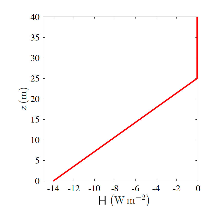
Fig. 21.8 Sensible heat flux.#
The profile is shown in Fig. 21.8. The upward turbulent flux is more positive (i.e. less negative) at higher \(z\). Therefore, more heat is transported out of a control volume than inward. This results in cooling.
The divergence of the vertical heat flux is equal to
This corresponds to a cooling term in the conservation equation of the boundary layer of 1.64 K hr\(^{-1}\).
d) By using the value found in b) and taking now into account the turbulent divergence term, calculate the temperature change per hour.
Answer
e) If now we consider in the budget equation for the temperature, the horizontal advection term \(U~\pafg{\overline{\theta}}{x}\). If \(U=10~m/s\), calculate the horizontal gradient of temperature (\(\pafg{\overline{\theta}}{x}\)) in order to reach a steady-state.
Answer
The horizontal advection has to balance the cooling effects of both the vertical heat flux gradient and the radiation. Therefore,
Since \(\overline{U}=10\rm\,m\,s^{-1}\), \(\gemafg{\theta}{x} \approx -1\cdot 10^{-4}\rm\,K\,m^{-1}\). This results in \(\gemafg{\theta}{x}=-0.1\rm\,K\,km^{-1}\)
Since the value is negative, relatively warm air is transported in the positive \(x\) direction and, consequently, advection is a source of heating.