18. Exercises week 2

\(\def\pafg#1#2{\dfrac{\partial #1}{\partial #2}}\) \(\def\afg#1#2{\dfrac{{\rm d} #1}{{\rm d} #2}}\)

18.1.

Given a surface specific humidity of 15 g/kg, a surface pressure of 1003 hPa and a temperature described by \( T = 4x + zy ~(C) \) calculate the potential temperature and the virtual potential temperature at the point (5, 1, 2) and at the pressure 850 hPa (\(R_d=287\ J\ Kg^{-1}\ K^{-1}, c_p=1004\ J\ Kg^{-1}\ K^{-1}\)).

Hint

\[\begin{split} \theta &= T\left(\frac{P_0}{P}\right)^{\frac{R_d}{c_p}}\\ \theta_v &= \theta \left(1 + 0.61 q \right) \end{split}\]

Answer

We know:

\[\begin{split} T(5,1,2) &= 4\cdot 5+2\cdot 1\,^\circ{\rm C}\\ &= 295\,{\rm K}\\ P_0 &= 1003\,{\rm hPa}\\ P &= 850\,{\rm hPa}\\ R_d &= 287\,{\rm J\,kg^{-1}\,K^{-1}}\\ c_p &= 1004\,{\rm J\,kg^{-1}\,K^{-1}}\\ q &= 15 \cdot 10^{-3}\,kg\,kg^{-1} \end{split}\]

Substituting these numbers results in:

\[\begin{split} \theta &= 309.29\,{\rm K}\\ \theta_v &= 312.12\,{\rm K}\\ \end{split}\]

18.2.

During a measurement campaign the following vertical profile of potential temperature was measured at 14 UTC (see Fig. 18.1).

a) Name each of the layers indicated in the figures with the letters A, B, C and D

Answer

• A. Surface layer

• B. Mixed layer

• C. Entrainment zone/layer

• D. Free troposphere

b) Find the vertical gradient of temperature

\[ \pafg{\theta}{z}\sim\frac{\Delta \theta}{\Delta z} \]

for each of the layers above mentioned.

Answer

It depends on how you draw the schematic lines.

• A. \(\rm \frac{-1.5 K}{300 m} = -5\ K\ km^{-1}\)

• B. \(\rm \frac{0 K}{1100 m} = 0\ K\ km^{-1}\)

• C. \(\rm \frac{8 K}{350 m} = 23\ K\ km^{-1}\)

• D. \(\rm \frac{0.75 K}{400 m} = 1.9\ K\ km^{-1}\)

c) Indicate for each layer whether it is stable, neutral or unstable and whether it is turbulent or laminar.

Answer

• A. Unstable and turbulent

• B. Neutral and turbulent

• C. Stable, but turbulent

• D. Stable and laminar

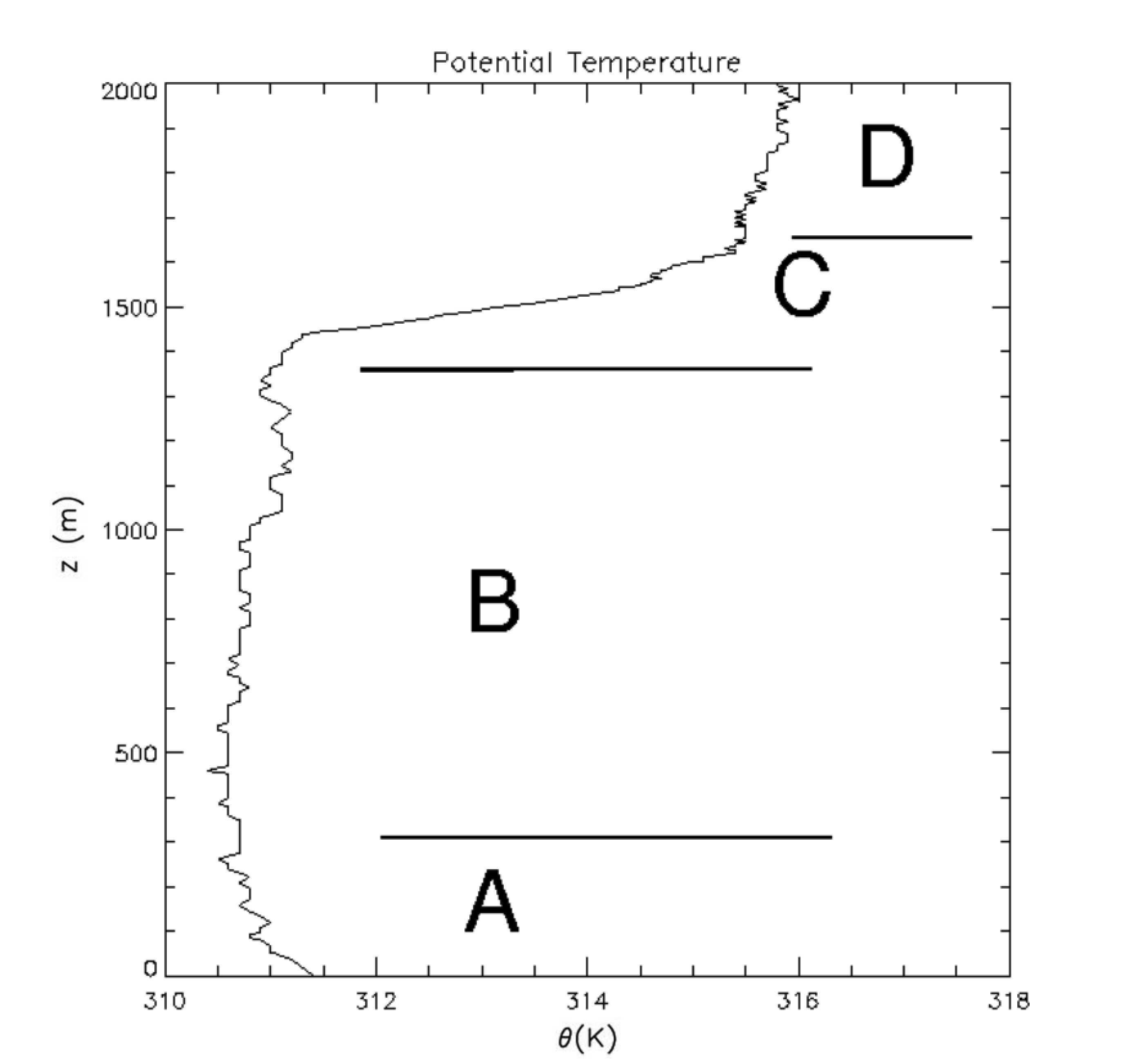
Fig. 18.1 Vertical profile of potential temperature measured by a radiosonde at 14 UTC.

18.3.

The Navier-Stokes equation for the horizontal, instantaneous velocity is

\[ \pafg{u_i}{t}+u_j\pafg{u_i}{x_j}~=~-\frac{1}{\rho}\pafg{p}{x_i}+f\epsilon_{ij3}u_j+\nu\pafg{^2 u_i}{x_j^2} \]

We can make this equation dimensionless by using the following (variables indicated with a \(*\) are dimensionless):

\(u_{i}^*= \dfrac{u_i}{\cal U}\)

\(x_{j}^*= \dfrac{x_j}{\cal L}\)

\(p^*= \dfrac{p}{\rho\, \cal U\rm^2}\)

\(\cal L\) and \(\cal U\) represent respectively the scaling height and scaling velocity.

a) Derive the dimensionless time variable (t*) by using t, \({\cal U}\) and \({\cal L}\)

Answer

The unit of time is seconds. To obtain something with the same units from \({\cal U}\) and \({\cal L}\), one can use \( \dfrac{\cal L}{\cal U}\) Therefore \(t^*= t\dfrac{\cal U}{\cal L}\)

b) Using the scales \(\cal U\), \(\cal L\), deduce the dimensionless form of the Navier Stokes equation.

Answer

\[\begin{split} u_i &= u_i^* \, \cal U\\ t &= t^* \, \frac{\cal L}{\cal U}\\ x_i &= x_i^* \, \cal L\\ p &= p^* \, \rho\, \cal U\rm^2\\ \end{split}\]

Substituting this in the Navier Stokes equations results in

\[\begin{split} \frac{\cal U\rm^2}{\cal L} \pafg{u_i^*}{t^*} + \frac{\cal U\rm^2}{\cal L} u_j^* \pafg{u_i^*}{x_j^*} = - \frac{\rho \cal U\rm^2}{\cal L} \frac{1}{\rho} \pafg{p^*}{x_i^*} + \cal U f \epsilon_{ij3}u_j^* + \frac{\cal U}{\cal L\rm^2} \nu \pafg{^2 u_i^*}{{x_j^*}^2}\\ \end{split}\]

This equation can be multiplied by \(\frac{\cal L}{\cal U\rm^2}\) to obtain the dimensionless form:

\[ \pafg{u_i^*}{t^*} + u_j^* \pafg{u_i^*}{x_j^*} = - \pafg{p^*}{x_i^*} + \frac{\cal L}{\cal U} f \epsilon_{ij3}u_j^* + \frac{\nu}{\cal U L} \pafg{^2 u_i^*}{{x_j^*}^2} \]

This can also be expressed with the Reynold’s number, \({\rm Re} = \frac{\cal U L}{\nu}\) and Rossby number \({\rm Ro} = \frac{\cal U}{f \cal L}\):

\[ \pafg{u_i^*}{t^*} + u_j^* \pafg{u_i^*}{x_j^*} = - \pafg{p^*}{x_i^*} + \frac{1}{\rm Ro} \epsilon_{ij3}u_j^* + \frac{1}{\rm Re} \pafg{^2 u_i^*}{{x_j^*}^2} \]

c) Typical length scales in the ABL are \(\cal U\)= 1 \(\rm{m\ s^{-1}}\) and \(\cal L\)=1000 m. Are the Coriolis rotational term and the viscous term relevant in the ABL?

(\(f=10^{-4}\ \rm{s^{-1}}\), \(\nu_{air}=1.5 \cdot 10^{-5}\ \rm{m^2\ s^{-1}}\))

Answer

Contribution of Coriolis force with respect to the other terms: \(f^* = f \frac{\cal L}{\cal U} = 0.1 = 10~\%\). This contribution is weak, but significant. Contribution of viscosity: \({\rm Re} = \frac{\cal U L}{\nu} = 6.7 \cdot 10^7\), so \(\frac{1}{\rm Re} \to 0\). This contribution is not significant. Consequently, this term can be neglected.

18.4.

The thermodynamic equation reads

\[ \pafg{\theta}{t}+u_j\pafg{\theta}{x_j} = \nu_{\theta}\pafg{^2\theta}{x_j^2} -\frac{1}{\rho c_p}\pafg{Q_j}{x_j}-\frac{L_vE}{\rho c_p} \]

a) Find the equation for the averaged potential temperature \(\overline{\theta}\).

Answer

\[\begin{split} \underbrace{\pafg{\theta}{t}}_{\rm Tendency} + \underbrace{u_j \pafg{\theta}{x_j}}_{\rm Advection} = \underbrace{\nu_{\theta}\pafg{^2\theta}{{x_j}^2}}_{\rm Viscosity} - \underbrace{\frac{1}{\rho c_p} \pafg{Q_j}{x_j}}_{\rm Radiation} - \underbrace{\frac{L_v E}{\rho c_p}}_{\rm Phase\,changes} \\ \pafg{\overline{\theta}}{t} + \overline{u_j \pafg{\theta}{x_j}} = \overline{\nu_{\theta}\pafg{^2\theta}{{x_j}^2}} - \overline{\frac{1}{\rho c_p} \pafg{Q_j}{x_j}} - \overline{\frac{L_v E}{\rho c_p}} \\ \pafg{\overline{\theta}}{t} + \overline{u_j}\,\overline{\pafg{\theta}{x_j}} + \overline{u_j' \pafg{\theta'}{x_j}} = \nu_{\theta}\pafg{^2\overline{\theta}}{{x_j}^2} - \frac{1}{\rho c_p} \pafg{\overline{Q_j}}{x_j} - \frac{L_v \overline{E}}{\rho c_p} \end{split}\]

Because of incompressibility, \(\pafg{u_j}{x_j}=0\), and therefore also \(\pafg{\overline{u_j}}{x_j}=\pafg{u_j'}{x_j} =0\). Therefore

(18.1)\[\begin{split} u_j'\pafg{\theta'}{x_j} &= u_j'\pafg{\theta'}{x_j} + \pafg{u_j'}{x_j} \theta' \\ &= \pafg{u_j'\theta'}{x_j} \end{split}\]

This is the flux form; after Reynolds averaging Equation (18.1), the divergence of a turbulent flux is obtained. Using this relation, the total thermodynamic equation reads

\[ \pafg{\overline{\theta}}{t} + \overline{u_j}\pafg{\overline{\theta}}{x_j} + \pafg{\overline{u_j'\theta'}}{x_j} = \nu_{\theta}\pafg{^2\overline{\theta}}{{x_j}^2}-\frac{1}{\rho c_p} \pafg{\overline{Q_j}}{x_j} - \frac{L_v \overline{E}}{\rho c_p} \]

b) Suppose that \(\overline{w'\theta'}~=~a - bz\) where \(a=0.3\ \rm{K\ m\ s^{-1}}\) and \(b=3 \cdot 10^{-4}\ \rm{K\ s^{-1}}\). How long will it take the ABL to warm up 0.54 K?

Hint

From the \(\overline{\theta}\) equation neglect subsidence, radiation and latent heat releases and assume horizontal homogeneity.

Answer

Since there are no clouds, no latent heat release is present: \(\overline{E}=0\).

The impact of radiation is relatively small during day: \(\frac{1}{\rho c_p} \pafg{\overline{Q_j}}{x_j} \approx 0\).

Due to the high turbulent nature of the atmospheric boundary layer, the viscous term can be neglected as well: \(\nu_{\theta}\pafg{^2\overline{\theta}}{{x_j}^2} \approx 0\).

We assume horizontal homogeneity, so \(x\) and \(y\) derivatives of Reynold’s averaged variables are equal to 0.

Without subsidence, the mean vertical wind velocity, \(\overline{w}\), is equal to 0 as well.

Finally, the equation results in

\[ \pafg{\overline{\theta}}{t} = - \pafg{\overline{w'\theta'}}{z} \]

Since \(\pafg{\overline{w'\theta'}}{z} = - b\), \(\pafg{\overline{\theta}}{t} = 3 \cdot 10^{-4}\rm\,K\,s^{-1}\). The time needed is equal to \(\frac{0.54\rm\,K}{3 \cdot 10^{-4}\rm\,K\,s^{-1}} = 1800\,{\rm s} = \frac{1}{2}\,{\rm hr}\).

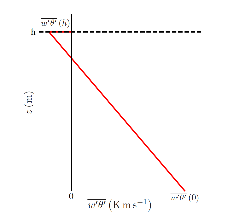
c) In a pseudo-stationary state, the vertical profile of the averaged potential temperature is constant with time, i.e. \(\left(\pafg{}{t}\right)\ \left(\pafg{\overline \theta}{z}\right) \approx 0\). Calculate the heat flux profile \(\overline {w'\theta'}(z)\) for the following boundary condition values of the heat flux at \(z=0~~\) \(\overline {w'\theta'}(0)\) and at \(z=h~~\) \(\overline {w'\theta'}(h)\).

Hint

Use the same assumptions as in 3b.

Answer

The governing equation is

\[ \pafg{\overline{\theta}}{t} = - \pafg{\overline{w'\theta'}}{z} \]

By taking the derivative to \(z\) of this equation, we obtain

(18.2)\[ \pafg{}{z}\left(\pafg{\overline{\theta}}{t}\right) = - \pafg{^2\overline{w'\theta'}}{z^2} \]

The left hand side can be rewritten:

(18.3)\[ \pafg{}{z}\left(\pafg{\overline{\theta}}{t}\right) = \pafg{}{t}\left(\pafg{\overline{\theta}}{z}\right) \approx 0 \]

This is known as the quasi-steady approximation. It holds true under convective conditions and states that the gradient of potential temperature does not change on time.

Equations (18.2) and (18.3) show that

\[\begin{split} \pafg{^2\overline{w'\theta'}}{z^2} &\approx 0\\ \end{split}\]

This results in

\[\begin{split} \pafg{\overline{w'\theta'}}{z} &= C_1 \\ \overline{w'\theta'} &= C_1 z + C_2 \end{split}\]

Using the boundary conditions:

\(\overline{w'\theta'} = \overline{w'\theta'}(0) + \left( \overline{w'\theta'}(h) - \overline{w'\theta'}(0) \right)\frac{z}{h}\)

In the figure, a visual representation is shown.

18.5.

The Bowen ratio is defined as the ratio of the heat flux to the moisture flux (\(B=H/LE\)). Using K-theory to parameterize the fluxes and assuming that \(K_h=K_q\), calculate the Bowen ratio from the following measurements at 10 meters (\(\theta=300\ \rm{K}\), \(q = 10\ \rm{g\ kg^{-1}}\)) and at 2 m (\(\theta=302\ \rm{K}\), \(q = 12\ \rm{g\ kg^{-1}}\)).

(\(L=2.5 \cdot 10^{6}\ \rm{J\ kg^{-1}}\) and \(c_p=1004\ \rm{J\ kg^{-1}\ K^{-1}}\))

Answer

\[ B=\frac{H}{LE} \]

We know

\[\begin{split} H &= \rho c_p \overline{w'\theta '}\\ LE &= \rho L \overline{w'q'}, \end{split}\]

which can be related to gradients using the first-order closure,

\[\begin{split} \overline{w'\theta '} &= - K_h \pafg{\overline{\theta}}{z} \\ \overline{w'q'} &= - K_q \pafg{\overline{q}}{z} . \end{split}\]

Therefore,

\[\begin{split} B &= \frac{\rho c_p \overline{w'\theta '}}{\rho L \overline{w'q'}} \\ &= \frac{c_p}{L} \frac{K_h}{K_q} \frac{\pafg{\overline{\theta}}{z}}{\pafg{\overline{q}}{z}} . \end{split}\]

All constants are known and from measurements follow \(\pafg{\overline{\theta}}{z} = \frac{-2\,{\rm K}}{8\,{\rm m}}\) and \(\pafg{\overline{q}}{z} = \frac{-2\cdot 10^{-3} \,{\rm kg\ kg^{-1}}}{8\,{\rm m}}\).

This results in B=0.4.

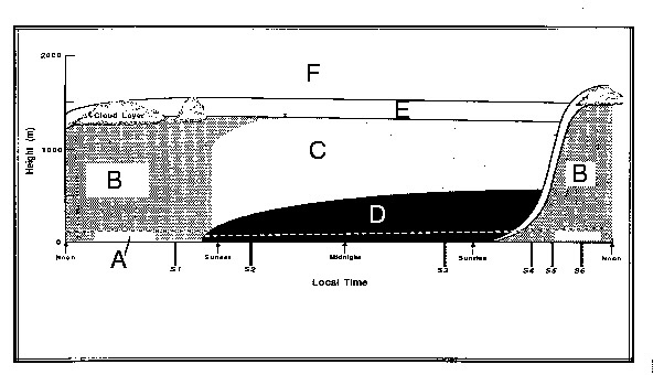
18.6.

Given the following draw of the evolution of the atmospheric Boundary Layer, fill in the table with the most appropriate labels (some examples have been already inserted) .

Region	Name	Lapse rate	Heat Flux	Static stability	Turbulent?
A		Superadiabatic
B	Mixed Layer
C			0
D					Sporadic
E		Subadiabatic		Stable
F					Sporadic

Answer

Region	Name	Lapse rate	Heat Flux	Static stability	Turbulent?
A	Surface Layer	Superadiabatic	>0	Unstable	Yes
B	Mixed Layer	Adiabatic	\(\begin{cases} >0 \\ <0 \end{cases} \)	Neutral	Yes
C	Residual layer	Adiabatic	0	Neutral	Sporadic
D	Nocturnal boundary layer	Subadiabatic	<0	Stable	Sporadic
E	Capping inversion	Subadiabatic	0	Stable	Sporadic
F	Free atmosphere	Subadiabatic	0	Stable	Sporadic

Superadiabatic: The temperature decreases more with height compared to the case of adiabatic cooling.

Subadiabatic: The temperature decreases less with height compared to the case of adiabatic cooling.

In the mixed layer, the heat flux decreases with height. It’s positive in the lower \(\frac{5}{6}\) part of the boundary layer and negative in the rest.

In the residual layer, capping inversion, and in the nocturnal boundary layer, turbulence is generated by shear. In the free troposphere as well, but less frequent due to the stronger stability.