17. Exercises week 1

Hint

At some exercises we provide hints. These can contains tips to help you find the answer, but they can also contain additional information. So, if you managed to answer the question without looking at the tip: great! But please also check the tip, because there might still be valuable information there.

\(\def\pafg#1#2{\dfrac{\partial #1}{\partial #2}}\) \(\def\afg#1#2{\dfrac{{\rm d} #1}{{\rm d} #2}}\)

17.1.

Calculate the Reynolds number of the following flows \((\nu_{air}=1.5\cdot10^{-5}\ \rm{m^{2}\ s^{-1}}, \nu_{water}=1.0\cdot10^{-6}\ \rm{m^{2}\ s^{-1}}, \nu_{blood}=3.8\cdot10^{-6}\ \rm{m^{2}\ s^{-1}})\). Classify if these flows are laminar or turbulent.

Hint

The Reynolds number is a dimensionless number, which is used to compare inertial forces with viscous forces. By comparing the magnitudes of those forces we can see how turbulent a flow is.

\[ {\rm Re} = \frac{U\cdot L}{\nu} \]

A laminar boundary layer flow becomes turbulent for \({\rm Re} \geq 5\cdot 10^5\). For other configurations, turbulent and laminar regimes are characterized by different regions, but in general, for \({\rm Re} < 10^3\), the flow is laminar and for \({\rm Re} > 10^5\) the flow is turbulent.

a) Atmospheric convective boundary layer (W=1 \(\mathrm{m\ s^{-1}}\), L=1000 m)

Answer

\[\begin{split} \left\lbrace U,L,\nu \right\rbrace &= \left\lbrace 1\,{\rm m\,s^{-1}},1000\,{\rm m},1.5\cdot 10^{-5}\,\rm{m^2\,s^{-1}} \right\rbrace\\ {\rm Re} &= 6.67\cdot 10^7 \end{split}\]

Turbulent

b) Oceanic internal waves (U = 0.05 \(\rm{m\ s^{-1}}\), L= 10000 m)

Answer

\[\begin{split} \left\lbrace U,L,\nu \right\rbrace &= \left\lbrace 0.05\,{\rm m\,s^{-1}},1\cdot 10^4\,{\rm m},1\cdot 10^{-6}\,\rm{m^2\,s^{-1}} \right\rbrace\\ {\rm Re} &= 5\cdot 10^8 \end{split}\]

Turbulent

c) Blood circulation ( U = 0.3 \(\rm{m\ s^{-1}}\), L= 0.01 m)

Answer

\[\begin{split} \left\lbrace U,L,\nu \right\rbrace &= \left\lbrace 0.30\,{\rm m\,s^{-1}},0.01\,{\rm m},3.8\cdot 10^{-6}\,\rm{m^2\,s^{-1}} \right\rbrace\\ {\rm Re} &= 789 \end{split}\]

Laminar

17.2.

The velocity and the temperature fields of a flow are given by:

\[ \vec U=(2x^2, xy, \ln(x)+zy)~(\rm{m\ s^{-1}}) ~~~~~~ T = 4x + zy ~(C) \]

a) Calculate the temperature gradient at the point (0, 1, 1).

Hint

Gradient of \(T = \pafg{}{x_i}T\)

Answer

\[\begin{split} \pafg{}{x_i}T\vert_{x=0,y=1,z=1} &= \left(\pafg{T}{x},\pafg{T}{y},\pafg{T}{z}\right)\vert_{x=0,y=1,z=1}\\ &= \left(4,z,y\right) \vert_{x=0,y=1,z=1}\\ &= \left(4,1,1\right) \end{split}\]

b) Calculate the velocity divergence at the point (-1, 5, 0). Is it a incompressible or compressible flow at this point?

Hint

Divergence of \(\bf U = \pafg{U_i}{x_i}\)

Answer

\[\begin{split} \pafg{\vec U_i}{x_i}\vert_{x=-1,y=5,z=0} &= \pafg{u}{x} + \pafg{v}{y} + \pafg{w}{z}\vert_{x=-1,y=5,z=0} \\ &= 4x + x + y\vert_{x=-1,y=5,z=0} \\ &= 0 \end{split}\]

Therefore, the flow could be incompressible at this point. However, the general flow field is compressible, since the divergence is only 0 only for \(y=-5x\)

17.3.

Let \(c\) be a constant, \(t\) a function of time and \(A\) and \(B\) turbulent variables. Expand the following terms into a mean and turbulent parts and apply Reynolds rules to simplify the expressions as much as possible.

Hint

For arbitrary variables, \(A\) and \(B\), and constants, \(c\), it holds that

\[\begin{split} \overline{c} &= c \\ \overline{c\,A} &= c\,\overline{A} \\ \overline{\overline{A}} &= \overline{A}\\ \overline{\overline{A}\,B} &= \overline{A} \, \overline{B} \\ \overline{A+B} &= \overline{A} + \overline{B}\\ \overline{\afg{A}{t}} &= \afg{\overline{A}}{t} \label{for:Rey6} \end{split}\]

The last equation also holds true for derivatives to other coordinates than \(t\), like \(x\), \(y\) and \(z\).

a) \(\overline{cAB}\)

Answer

\[\begin{split} \overline{cAB} &= c \overline{AB}\\ &=c\overline{\left(\overline{A}+A'\right)\left(\overline{B}+B'\right)}\\ &=c\overline{\left(\overline{A}\,\overline{B}+\overline{A}B'+A'\overline{B}+A'B'\right)}\\ &=c\left(\overline{\overline{A}\,\overline{B}}+\overline{\overline{A}B'}+\overline{A'\overline{B}}+\overline{A'B'}\right)\\ &=c\left(\overline{A}\,\overline{\overline{B}}+\overline{A}\,\overline{B'}+\overline{B}\,\overline{A'}+\overline{A'B'}\right)\\ &=c\left(\overline{A}\,\overline{B}+\overline{A'B'}\right) \end{split}\]

b) \(\overline{A\pafg{B}{t}}\)

Answer

Consider \(C \equiv \pafg{B}{t}\), so according to the averaging rules: \(\overline{C} = \overline{\pafg{B}{t}} = \pafg{\overline{B}}{t}\) and \(C' = C - \overline{C} = \pafg{B}{t} - \pafg{\overline{B}}{t} = \pafg{B-\overline{B}}{t} = \pafg{B'}{t}\)

\[\begin{split} \overline{A\pafg{B}{t}} &= \overline{AC}\\ &= \overline{\left(\overline{A}+A'\right)\left(\overline{C}+C'\right)}\\ &=\overline{\left(\overline{A}\,\overline{C}+\overline{A}C'+A'\overline{C}+A'C'\right)}\\ &=\left(\overline{\overline{A}\,\overline{C}}+\overline{\overline{A}C'}+\overline{A'\overline{C}}+\overline{A'C'}\right)\\ &=\left(\overline{A}\,\overline{\overline{C}}+\overline{A}\,\overline{C'}+\overline{C}\,\overline{A'}+\overline{A'C'}\right)\\ &= \overline{A}\,\overline{C}+\overline{A'C'}\\ &= \overline{A}\pafg{\overline{B}}{t}+\overline{A'\pafg{B'}{t}} \end{split}\]

c) \(\overline{\pafg{A}{t}\pafg{B}{t}}\)

Answer

Same strategy as the one in solution b, only now also consider \(D \equiv \pafg{A}{t}\) with the same rules. (\(\overline{D} = \pafg{\overline{A}}{t}\) and \(D' = \pafg{A'}{t}\)).

\[\begin{split} \overline{\pafg{A}{t}\pafg{B}{t}} &= \overline{DC}\\ &= \overline{\left(\overline{D}+D'\right)\left(\overline{C}+C'\right)}\\ &=\overline{\left(\overline{D}\,\overline{C}+\overline{D}C'+D'\overline{C}+D'C'\right)}\\ &=\left(\overline{\overline{D}\,\overline{C}}+\overline{\overline{D}C'}+\overline{D'\overline{C}}+\overline{D'C'}\right)\\ &=\left(\overline{D}\,\overline{\overline{C}}+\overline{D}\,\overline{C'}+\overline{C}\,\overline{D'}+\overline{D'C'}\right)\\ &= \overline{D}\,\overline{C}+\overline{D'C'}\\ &= \pafg{\overline{A}}{t}\pafg{\overline{B}}{t}+\overline{\pafg{A'}{t}\pafg{B'}{t}} \end{split}\]

17.4.

The following terms are given in summation notation. Expand them (that is, write out each term of the indicated sums).

a) \(\pafg{\overline{u_i'u_j'}}{x_j}\)

Answer

\[ \pafg{\overline{u_i'u_j'}}{x_j}=\pafg{\overline{u_i'u'}}{x}+\pafg{\overline{u_i'v'}}{y}+\pafg{\overline{u_i'w'}}{z} \]

This can be further expanded to:

\[ \pafg{\overline{u_i'u_j'}}{x_j}=\left( \pafg{\overline{u'u'}}{x}+\pafg{\overline{u'v'}}{y}+\pafg{\overline{u'w'}}{z} , \pafg{\overline{v'u'}}{x}+\pafg{\overline{v'v'}}{y}+\pafg{\overline{v'w'}}{z} , \pafg{\overline{w'u'}}{x}+\pafg{\overline{w'v'}}{y}+\pafg{\overline{w'w'}}{z} \right) \]

b) \( u_i'\pafg{\theta'}{x_i} \)

Answer

\[ u_i'\pafg{\theta'}{x_i} = u'\pafg{\theta'}{x} + v'\pafg{\theta'}{y} + w'\pafg{\theta'}{z} \]

c) \( \overline{u_j} \pafg{\overline{u_i'u_k'}}{x_j} \)

Answer

\[ \overline{u_j}\pafg{\overline{u_i'u_k'}}{x_j} = \overline{u}\pafg{\overline{u_i'u_k'}}{x} + \overline{v}\pafg{\overline{u_i'u_k'}}{y} + \overline{w}\pafg{\overline{u_i'u_k'}}{z} \]

This can be further expanded to:

\[\begin{split} \overline{u_j}\pafg{\overline{u_i'u_k'}}{x_j} &= \left(\overline{u}\pafg{}{x}+\overline{v}\pafg{}{y}+\overline{w}\pafg{}{z}\right)\overline{u_i'u_k'}\\ &= \left(\overline{u}\pafg{}{x}+\overline{v}\pafg{}{y}+\overline{w}\pafg{}{z}\right)\left [\begin{matrix} \overline{u'u'} & \overline{u'v'} & \overline{u'w'} \\ \overline{v'u'} & \overline{v'v'} & \overline{v'w'} \\ \overline{w'u'} & \overline{w'v'} & \overline{w'w'}\\ \end{matrix}\right] \end{split}\]

d) \( \delta_{i3}g \)

Answer

No double indicators, so the summation cannot be performed. However, it can be further expanded to:

\[ \delta_{i3}g = \left(0,0,g\right) \]

This term is present in the Navier-Stokes equation. It tells us that only the 3\(^{\rm rd}\) dimension of the vector (usually \(w\)) is affected by gravity and, consequently, buoyancy.

e) \( \pafg{\tau_{mn}}{x_n} \)

Answer

\[ \pafg{\tau_{mn}}{x_n} = \pafg{\tau_{m1}}{x} + \pafg{\tau_{m2}}{y} + \pafg{\tau_{m3}}{z} \]

since indices 1, 2 and 3 correspond to the \(x\), \(y\) and \(z\) coordinates, respectively. This can be further expanded to:

\[ \pafg{\tau_{mn}}{x_n} = \left( \pafg{\tau_{11}}{x} + \pafg{\tau_{12}}{y} + \pafg{\tau_{13}}{z} , \pafg{\tau_{21}}{x} + \pafg{\tau_{22}}{y} + \pafg{\tau_{23}}{z} , \pafg{\tau_{31}}{x} + \pafg{\tau_{32}}{y} + \pafg{\tau_{33}}{z} \right) \]

17.5.

With a frequency of 1 Hz and during 8 seconds we have measured the following values of the vertical velocity and specific humidity

t [s]	0	1	2	3	4	5	6	7
\(w\ \rm(m\ s^{-1})\)	0	-2	-1	1	-2	2	1	1
\(q\ \rm(g\ kg^{-1})\)	8	9	9	6	10	3	5	6

a) Calculate the time average of \(w\) and \(q\)

Answer

\(\overline{w} = 0\rm\,m\,s^{-1}\) and \(\overline{q} = 7 \rm\,g\,kg^{-1}\).

b) Calculate the moisture flux. What is the direction of the flux?

Answer

t [s]	0	1	2	3	4	5	6	7
\(q'\ \mathrm{[g\ kg^{-1}]}\)	1	2	2	-1	3	-4	-2	-1
\(w'\ \mathrm{[m\ s^{-1}]}\)	0	-2	-1	1	-2	2	1	1
\(w'q'\ \mathrm{[g\ kg^{-1}\ m\ s^{-1}]}\)	0	-4	-2	-1	-6	-8	-2	-1

Therefore, \(\overline{w'q'} = -3 \rm \,g\,kg^{-1}\,m\,s^{-1}\). The moisture flux is directed downward.

c) Calculate the vertical velocity and specific humidity variances

Answer

t [s]	0	1	2	3	4	5	6	7
\(q'^2\ \mathrm{[g^2\,kg^{-2}]}\)	1	4	4	1	9	16	4	1
\(w'^2\ \rm \,[m^2\,s^{-2}]\)	0	4	1	1	4	4	1	1

So, \(\sigma_w^2 \equiv \overline{w'^2} = 2 \rm\,m^2\,s^{-2}\) and \(\sigma_q^2 \equiv \overline{q'^2} = 5 \rm\,g^2\,kg^{-2}\).

17.6.

We have measured in a meteorological mast the following values for the wind: \(\rm{\overline{u}}\)(2 m)= 2.8 \(\rm{m\ s^{-1}}\) and \(\rm{\overline{u}}\)(20 m) = 5.75 \(\rm{m\ s^{-1}}\).

a) Calculating using linear interpolation the value of the wind at 9 m.

Answer

\[ \overline{u}(z) = \frac{z-z_1}{z_2-z_1}\left(\overline{u}(z_2)-\overline{u}(z_1)\right) + \overline{u}(z_1) \]

\(z_1=2\,\rm m\), \(z_2=20\,\rm m\), \(\overline{u}(z_1)=2.8\,\rm m\,s^{-1}\) and \(\overline{u}(z_2)=5.75\,\rm m\,s^{-1}\). Therefore \(\overline{u}\rm\left(9\, m\right) = 3.95\,m\,s^{-1}\).

b) If the wind velocity gradient reads:

\[ \pafg{\overline{u}}{z}=\frac{u_*}{\kappa~z}. \]

Assuming the following values for the friction velocity (=0.5 \(\rm{m\ s^{-1}}\)), the roughness length (= 0.2 m) and the Von Karman constant (=0.4), calculate the wind speed at 9 m.

Answer

According to this equation, we get a logarithmic wind profile. This can be used in two ways: starting from \(z=z_0\) or from \(z=z_1=2\,\rm m\). Both will be explored here.

\[\begin{split} \pafg{\overline{u}}{z} &= \frac{u_*}{\kappa z} \\ \partial \overline{u} &= \frac{u_*}{\kappa} \frac{\partial z}{z} \end{split}\]

This can be integrated:

\[\begin{split} \int_{\overline{u}\left({z_1}\right)}^{\overline{u}\left({z_2}\right)} {\rm d} \overline{u} &= \int_{z_1}^{z_2} \frac{u_*}{\kappa} \frac{{\rm d} z}{z}\\ &= \frac{u_*}{\kappa} \int_{z_1}^{z_2} \frac{1}{z} {\rm d} z \end{split}\]

This results in:

\[\begin{split} \overline{u}|_{\overline{u}\left({z_2}\right)} - \overline{u}|_{\overline{u}\left({z_1}\right)} &= \frac{u_*}{\kappa} \left(\ln z|_{z_2} - \ln z|_{z_1}\right)\\ \overline{u}(z'_2) &= \overline{u}(z'_1) + \frac{u_*}{\kappa} \ln \left(\frac{z'_2}{z'_1}\right) \end{split}\]

in which \(z'_1\) and \(z'_2\) are two arbitrary heights. In both cases \(z'_2 = 9\,\rm m\) and also \(u_* = 0.5\,\rm m\,s^{-1}\) and \(\kappa=0.4\).

In the first situation, \(z'_1=z_0=0.2\,\rm m\) with the corresponding wind velocity \(\overline{u}(z'_1) = 0\,\rm m\,s^{-1}\). In this case \(\overline{u}(9\,\rm m) = 4.76\,\rm m\,s^{-1}\).

In the second situation,\(z'_1=z_1=2\,\rm m\) with the corresponding wind velocity \(\overline{u}(z'_1) = 2.8\,\rm m\,s^{-1}\). In this case \(\overline{u}(9\,\rm m) = 4.68\,\rm m\,s^{-1}\).

c) Estimate the error associated to the calculation of the wind speed using the linear interpolation.

Answer

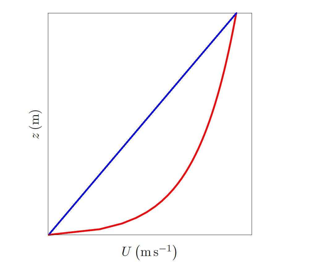
The figure shows the linear approximation from question a in blue and the logarithmic wind profile from question b in red. The error made with the linear interpolation is the difference between these lines.

At 9 m the estimation with the linear interpolation is \(\overline{u}\rm\left(9\, m\right) = 3.95\,m\,s^{-1}\).

Comparing the linear interpolation with the logarithmic profile in the first situation results in an error of \(0.81\,\rm m\,s^{-1}\).

Comparing the linear interpolation method with the logarithmic profile in the second situation results in an error of \(0.73\,\rm m\,s^{-1}\).

17.7.

The general momentum equations are:

\[\begin{split} \begin{cases} \pafg{u}{t} + u_j \pafg{u}{x_j} = f v - \dfrac{1}{\overline{\rho}}\pafg{p}{x}+ \nu \pafg{^2u}{{x_j}^2} \\ \pafg{v}{t} + u_j \pafg{v}{x_j} = - f u - \dfrac{1}{\overline{\rho}}\pafg{p}{y}+ \nu \pafg{^2v}{{x_j}^2} \end{cases} \end{split}\]

a) Simplify these equations by

• applying Reynolds averaging;

• considering \(\overline{w} = 0\), horizontal homogeneity of the wind and incompressibility;

• neglecting the small viscosity term;

• assuming that at larger scales the Coriolis force and horizontal pressure gradients balance to reach a geostrophic wind.

Answer

Reynold’s averaging results in

\[\begin{split} \begin{cases} \pafg{\overline{u}}{t} + \overline{u_j} \pafg{\overline{u}}{x_j} + \overline{u_j'\pafg{{u'}}{x_j}} = f \overline{v} - \dfrac{1}{\overline{\rho}}\pafg{\overline{p}}{x}+ \nu \pafg{^2\overline{u}}{{x_j}^2} \\ \pafg{\overline{v}}{t} + \overline{u_j} \pafg{\overline{v}}{x_j} + \overline{u_j'\pafg{{v'}}{x_j}} = - f \overline{u} - \dfrac{1}{\overline{\rho}}\pafg{\overline{p}}{y}+ \nu \pafg{^2\overline{v}}{{x_j}^2} \end{cases} \end{split}\]

Considering \(\overline{w} = 0\),

horizontal homogeneity of the wind(\(\pafg{\chi}{x}=\pafg{\chi}{y}=0\) with \(\chi\) as u, v),

incompressibility (\(\pafg{u_i'}{x_i}=0\)),

and the chain rule (\(\pafg{u_i\chi}{x_i}\)=\(u_i\pafg{\chi}{x_i}+\pafg{u_i}{x_i}\chi\)),

this results in

\[\begin{split} \begin{cases} \pafg{\overline{u}}{t} + \pafg{\overline{u_j'u'}}{x_j} = f \overline{v} - \dfrac{1}{\overline{\rho}}\pafg{\overline{p}}{x}+ \nu \pafg{^2\overline{u}}{{x_j}^2} \\ \pafg{\overline{v}}{t} + \pafg{\overline{u_j'v'}}{x_j} = - f \overline{u} - \dfrac{1}{\overline{\rho}}\pafg{\overline{p}}{y}+ \nu \pafg{^2\overline{v}}{{x_j}^2} \end{cases} \end{split}\]

Neglecting the small viscosity term (for high Reynolds numbers) and assuming that at larger scales the Coriolis force and horizontal pressure gradients balance to reach a geostrophic wind, \(\dfrac{1}{\overline{\rho}}\pafg{\overline{p}}{x} = f v_g\) and \(\dfrac{1}{\overline{\rho}}\pafg{\overline{p}}{y} = -f u_g\), the momentum equations are:

\(\pafg{\overline{u}}{t} + \pafg{\overline{u'w'}}{z}\) = \(f \left(\overline{v}-v_g\right) \)

\(\pafg{\overline{v}}{t} + \pafg{\overline{v'w'}}{z}\) = \(-f \left(\overline{u}-u_g\right) \)

In this representation, \(u_g\) and \(v_g\) are components of the geostrophic wind, which is the steady state wind considering the horizontal pressure gradients and the Coriolis force.

b) Now suppose that \(\overline{u'w'}=-(u_*+cz)^2\) and \(\overline{v'w'}=0\) for all \(z\) and the geostrophic velocities for the x- and y-components are 5 \(\rm{m\ s^{-1}}\) and 5 \(\rm{m\ s^{-1}}\) at all heights, respectively.

Find the acceleration of air in the x- and y-directions \(\left(\pafg{\overline{u}}{t}, \pafg{\overline{v}}{t}\right)\) at a height of 100 m in the ABL. The initial velocities at 100 m are \(\overline{u}=\ 4\ \rm{m\ s^{-1}}\) and \(\overline{v}=\ 2\ \rm{m\ s^{-1}}\).

(\(u_* = 0.3\ \rm{m\ s^{-1}}\), \(f = 10^{-4}\ \rm{s^{-1}}\) and \(c = 10^{-3}\ \rm{s^{-1}}\)).

Answer

In this specific case, filling up the momentum fluxes, the governing equations for the acceleration are:

\[\begin{split} \pafg{\overline{u}}{t} &= 2 c \left(u_*+c z\right) + f \left(\overline{v}-v_g\right) \\ \pafg{\overline{v}}{t} &= -f \left(\overline{u}-u_g\right) \end{split}\]

Substituting the values, results in:

\(\pafg{\overline{u}}{t}\) = \(5 \cdot 10^{-4}\,\rm m\,s^{-2}\)

\(\pafg{\overline{v}}{t}\) = \(1 \cdot 10^{-4}\,\rm m\,s^{-2}\)