20. Exercises week 4

\(\def\pafg#1#2{\dfrac{\partial #1}{\partial #2}}\) \(\def\afg#1#2{\dfrac{{\rm d} #1}{{\rm d} #2}}\) \(\def\gemafg#1#2{\pafg{\overline{#1}}{#2}}\)

Hint

Pay attention to the units!

20.1.

Fig. 20.1, Fig. 20.2, and Fig. 20.3 show the vertical profiles of the potential temperature measured by radiosondes in the USA at 11, 17 and 23 UTC the 20th June 1997 (local time=UTC-6 hours).

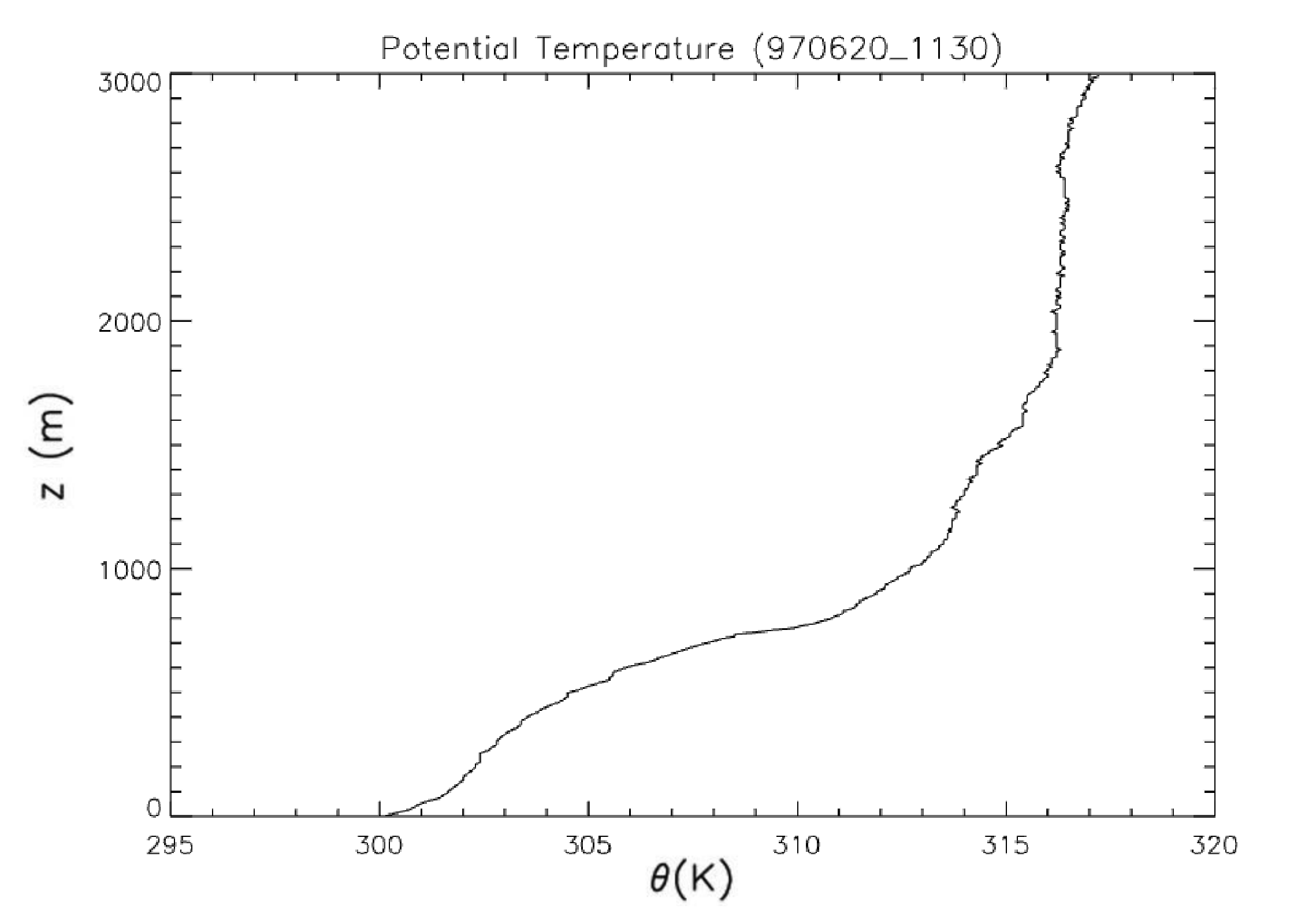
Fig. 20.1 Vertical profile of potential temperature measured by radiosondes at 11 UTC

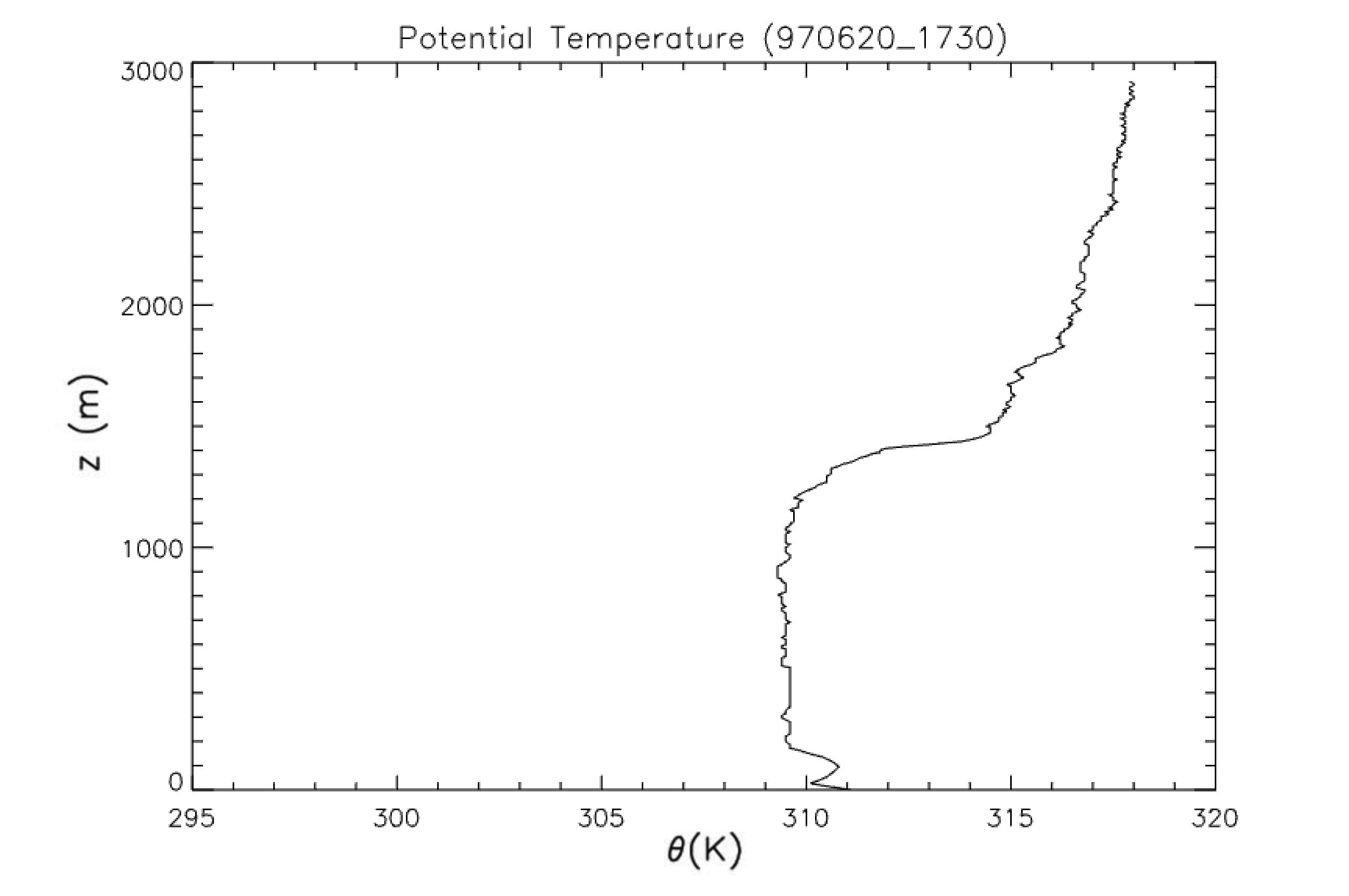
Fig. 20.2 Vertical profile of potential temperature measured by radiosondes at 17 UTC

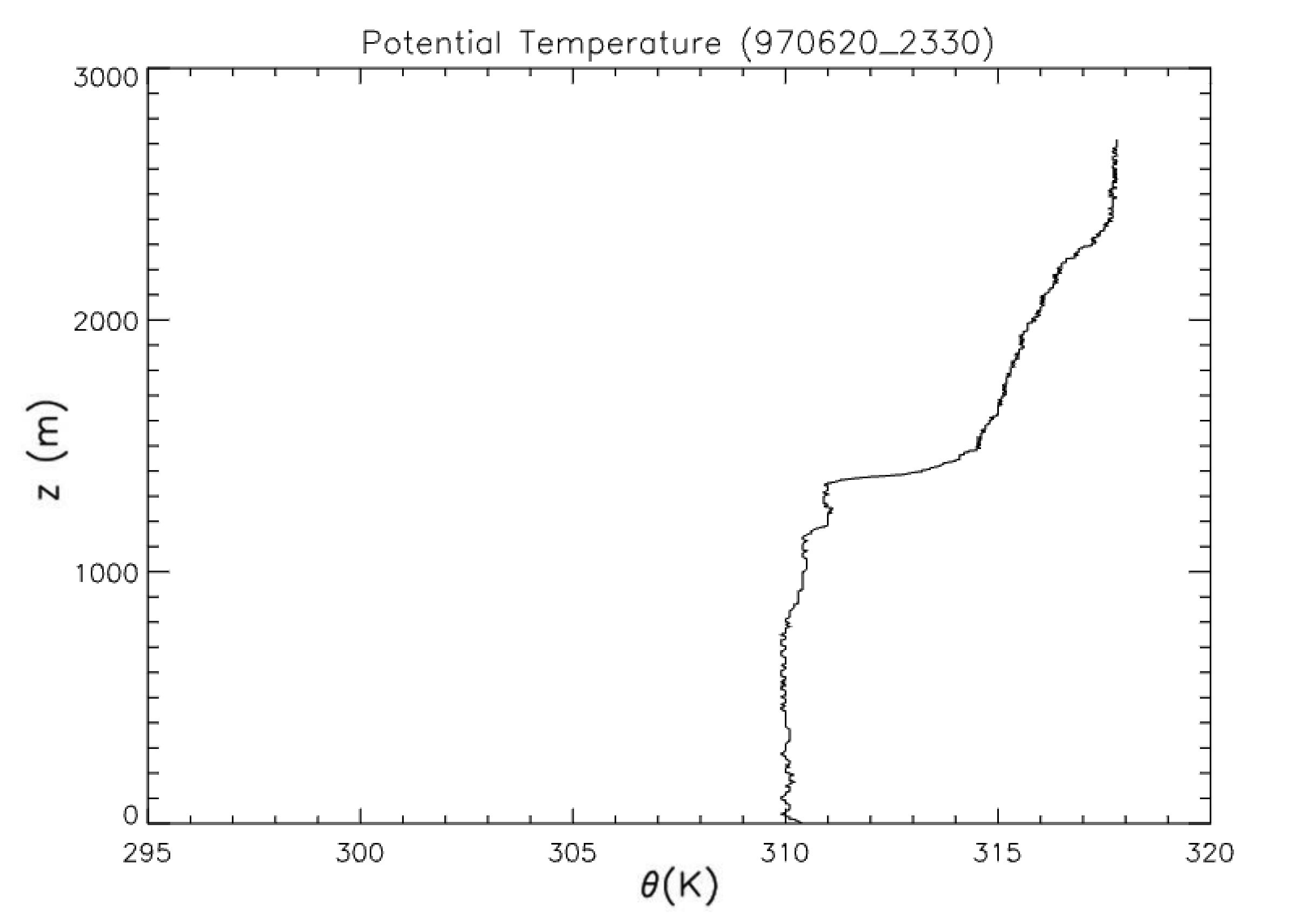
Fig. 20.3 Vertical profile of potential temperature measured by radiosondes at 23 UTC

a) Describe the radiosoundings by giving the boundary layer height, the mixed layer temperature, the temperature inversion and the laspe rate (h (m), \(\left<\theta\right>\) (K), \(\Delta\theta\) (K), \(\gamma_\theta\) (K km\(^{-1}\))).

Answer

Figure	Fig. 20.1	Fig. 20.2	Fig. 20.3
h (m)	700	1400	1400
\(\left<\theta\right>\) (K)	303	309.5	310
\(\Delta\theta\) (K)	9	5	4
\(\gamma_\theta\) (K km\(^{-1}\))	2.2	2.5	2.5

Note: The upper profile shows a stable boundary layer, while the other two profiles show well-mixed convective boundary layers.

b) Give the evolution of the boundary layer depth.

Answer

From 05.30 LT to 11.30 LT: + 700 m, so a growth of approximately 3 \(\rm{cm\ s^{-1}}\).

From 11.30 LT to 17.30 LT: the boundary layer height is constant, so a growth of 0 \(\rm{cm\ s^{-1}}\).

c) Assuming an entrainment velocity equal to 0.01 m/s, find the entrainment flux at 17 UTC.

Answer

At 17 UTC (11 LT), \(\Delta\theta=5\rm\,K\).

\[ \overline{w'\theta'(z_i)} = - w_e\,\Delta\theta \]

Substituting the variables results in \(\overline{w'\theta'(z_i)} = -0.05\rm\,K\,m\,s^{-1}\).

The flux is negative, since heat is transported downwards.

20.2.

During the 27th of July 2002, the vertical profile of potential temperature and heat flux (see Fig. 20.4 and Fig. 20.5) were measured by an aircraft above Cabauw. The heat flux measurements were taken around 12.45 UTC.

a) Estimate the boundary layer height at 8.15 UTC and 12.45. Calculate the velocity of the growth of the convective boundary layer.

Answer

Using the location where \(\pafg{\theta}{z}\) has its maximum, the boundary layer heights at 8.15 UTC and 12.45 UTC are 375 m and 1025 m, respectively. Therefore, the velocity of growth is \(\dfrac{650\rm\,m}{4.5\cdot 3600\rm\,s} = 0.04\rm\,m\,s^{-1}\).

b) Calculate the terms (storage, turbulent flux divergence) of the potential temperature equation.

Answer

\[ \gemafg{\theta}{t}+\gemafg{w'\theta'}{z} = {\rm Advection} + {\rm Sources/sinks} \]

Sources correspond with warming and sinks with cooling.

Storage term: \(\gemafg{\theta}{t} = \frac{5\rm\,K}{4.5\rm\,hr}=3.1\times 10^{-4}\rm\,K\,s^{-1}\)

Turbulent flux divergence: \(\gemafg{w'\theta'}{z} = \frac{-0.095\rm\,K\,m\,s^{-1}}{700\rm\,m}= -1.4\times 10^{-4}\rm\,K\,s^{-1}\)

c) Was the advection of potential temperature an important term during the 27th July 2002?

Answer

Since other sources and sinks are negligible during day, advection should account for the difference between storage and the vertical turbulent flux divergence. Therefore, advection should account for \(1.7\times 10^{-4}\rm\,K\,s^{-1}\). This is of the same order of magnitude as the temperature tendencies of the terms that are related to storage and transport by turbulent fluxes. This shows that advection is important for this case.

d) According to K-theory, the heat flux can be related to the gradient of the mean potential temperature as follows

\[ \overline{w'\theta'(z)}=-K_h\pafg{\overline{\theta}}{z} \]

Using the information from the vertical flux of potential temperature and heat flux, determine the exchange coefficient \(K_h\) at z=500 m (time 12.45). Discuss the result.

Answer

\[ \overline{w'\theta'(z)}=-K_h\pafg{\overline{\theta}}{z} \]

Rewritting this equation gives:

\[ K_h = - \dfrac{\overline{w'\theta'(z)}}{\pafg{\overline{\theta}}{z}} \]

From the graph, we note that at 500m \(\pafg{\overline{\theta}}{z} \approx 0\), this would result in \(K_h\ \to\infty\). This shows that local K-theory is not applicable in a well mixed boundary layer.

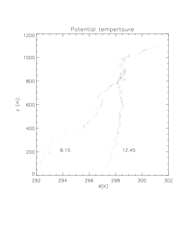
Fig. 20.4 Vertical profile of potential temperature measured above Cabauw during the 27th July 2002

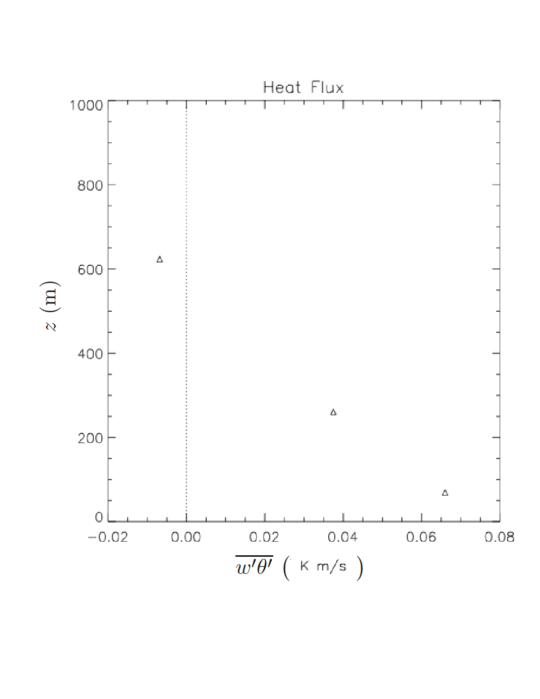
Fig. 20.5 Vertical profile of sensible heat flux measured above Cabauw during the 27th July 2002

20.3.

This exercise is about a convective boundary layer without any background wind. The strength of turbulent convection in such a boundary layer is related to the surface flux of virtual potential temperature \(\overline{w^\prime \theta_v^\prime}_0\) and its depth \(h\). We assume that the former is 0.1 K m s\(^{-1}\), and the latter is 1000 m. The kinematic viscosity \(\nu\) is \(1.5 \cdot 10^{-5}\) m\(^2\) s\(^{-1}\). The boundary layer is in quasi-steady state, which means that production and destruction by approximation balance. We assume that \(g / \overline{\theta}_v\) is 10 / 300.

a) What is the typical velocity \(w_*\) of a convective boundary layer, given its surface flux and depth and what is its value in this case?

Answer

The Deardorff velocity scale is constructed from \(\dfrac{g}{\overline{\theta}_v} \overline{w^\prime \theta^\prime}_0\) and \(h\). The only way to create a velocity scale is \(w_* \equiv \left( \dfrac{g}{\overline{\theta}_v} \overline{w^\prime \theta^\prime}_0 h \right)^\frac{1}{3}\). Its value here is 1.49 m s\(^{-1}\).

b) What is the Reynolds number of this convective boundary layer?

Answer

The Reynolds number here is \(Re = w_* h / \nu\) and its value is very close to \(1 \cdot 10^8\).

c) What is the typical magnitude of the production of turbulence in this system?

Answer

The production is the buoyancy term from TKE equation: \(\dfrac{g}{\overline{\theta}_v} \overline{w^\prime \theta_v^\prime}\). We take the surface value as a reference as this is where the energy enters the system: \(\dfrac{g}{\overline{\theta}_v} \overline{w^\prime \theta_v^\prime}_0\). Its value is \(3.33 \cdot 10^{-3}\) m\(^2\) \(s^{-3}\).

d) What is the magnitude of the dissipation of turbulence in this system?

Answer

The dissipation is approximately equal to the buoyancy term from TKE equation as there is almost steady state, hence its value is \(3.33 \cdot 10^{-3}\) m\(^2\) \(s^{-3}\).

e) What is the Kolmogorov scale of this convective boundary layer?

Answer

Dissipation matches the buoyancy flux, thus the Kolmogorov length \(\eta = \left( \nu^3 / \epsilon \right)^\frac{1}{4} = \left( \nu^3 / \dfrac{g}{\overline{\theta}_{v}} \overline{w^\prime \theta_v^\prime}_0 \right)^\frac{1}{4}\). Its value here is \(1.0 \cdot 10^{-3}\) m, thus one millimeter.

f) Show that the Reynolds number is proportional to \(\left( h / \eta \right)^\frac{4}{3}\).

Answer

\[\begin{split} \dfrac{h}{\eta} &= \dfrac{h}{\left( \nu^3 / \dfrac{g}{\overline{\theta}_{v}} \overline{w^\prime \theta_v^\prime}_0 \right)^\frac{1}{4}} \\ &= \dfrac{h \left( \dfrac{g}{\overline{\theta}_{v}} \overline{w^\prime \theta_v^\prime}_0 \right)^\frac{1}{4}} {\nu^\frac{3}{4}} \\ &= \dfrac{h^\frac{3}{4} h^\frac{1}{4} \left( \dfrac{g}{\overline{\theta}_{v}} \overline{w^\prime \theta_v^\prime}_0 \right)^\frac{1}{4}} {\nu^\frac{3}{4}} \\ &= \dfrac{h^\frac{3}{4} w_*^\frac{3}{4}} {\nu^\frac{3}{4}} \\ &= Re^\frac{3}{4} \end{split}\]

20.4.

The atmospheric boundary layer height is 300 m at 0600 UTC, the temperature lapse rate is 5 K/km and the initial temperature is \(\theta\) is 285 K . Assuming that the sensible heat flux varies with time over this land according to (t is given in hours):

\[\begin{split} \overline{w'\theta'(0)}&=c_1 \sin \left( \frac{\pi(t-t_0)}{c_2} \right ) \\ c_1&=0.2\ Km\ s{-1} \\ c_2&=12\ hours \end{split}\]

a) Under encroachment conditions, find the boundary layer height at 14 UTC, if the entrainment flux and subsidence are neglectable.

Answer

In case of encroachment:

\[\begin{split} \afg{\Delta\theta}{t} &= 0 \\ \gamma_{\theta}\afg{h}{t}- \afg{\left<\overline{\theta}\right>}{t} &= 0\\ \afg{h}{t} &= \frac{1}{\gamma_{\theta}}\afg{\left<\overline{\theta}\right>}{t} \end{split}\]

Since in the case of encroachment, \(\overline{w'\theta'}(h)=0\), Equation (20.6) becomes

\[ \afg{\left<\overline{\theta}\right>}{t} = \frac{\overline{w'\theta'}\left(0\right)}{h} \]

Therefore,

(20.1)\[ \afg{h}{t} = \frac{1}{\gamma_{\theta}}\frac{\overline{w'\theta'}_0}{h} \]

\[\begin{split} h\,\rm{d}h &= \frac{\overline{w'\theta'}_0}{\gamma_{\theta}} \rm{d}t\\ \int_{h_1}^{h_2}{h\ {\rm d}h} &= \int_{t1}^{t2}{\frac{\overline{w'\theta'}_0}{\gamma_{\theta}}{\rm d}t}\\ \dfrac{1}{2}\ h_2^2-\dfrac{1}{2}\ h_1^2 &= \frac{1}{\gamma_\theta} \int_{t1}^{t2}{\overline{w'\theta'}_0{\rm\,d}t} \end{split}\]

Finally,

\[ h_2 = \sqrt{h_1^2 + \frac{2}{\gamma_\theta} \int_{t1}^{t2}{\overline{w'\theta'}_0{\rm\,d}t}} \]

Substituting the heat flux results in

\[ h_2 = \sqrt{h_1^2 + \frac{2}{\gamma_\theta} \int_{t1}^{t2}{c_1 \sin\left(\frac{\pi\left(t-t_0\right)}{c_2}\right){\rm\,d}t}} \]

In this equation, the integral is given by

\[\begin{split} \int_{t1}^{t2}{c_1 \sin\left(\frac{\pi\left(t-t_0\right)}{c_2}\right){\rm\,d}t} &= c_1 \left[{-\frac{c_2}{\pi}\cos\left(\frac{\pi\left(t-t_0\right)}{c_2}\right)}\right]_{t_1}^{t_2}\\ &= \frac{c_1\,c_2}{\pi} \left({\cos\left(\frac{\pi\left(t_1-t_0\right)}{c_2}\right)-\cos\left(\frac{\pi\left(t_2-t_0\right)}{c_2}\right)}\right)_{t_1}^{t_2}\\ &\approx 4125 {\rm\,K\,m} \end{split}\]

for \(t_1=t_0=0600\rm\,UTC\) and \(t_2=1400\rm\,UTC\). Substituting this value, \(h_1\), \(c_1\) and \(c_2\) nets \(h\left(1400\rm\,UTC\right)\approx 1319\rm\,m\)

b) Calculate the boundary layer height at 14 UTC assuming that there is a closure assumption between the heat flux at the surface and at the entrainment zone:

\[ \overline{w'\theta'(z_i)}~=~-\beta \overline{w'\theta'(0)}, \]

where \(\beta\) is 0.2.

Answer

This exercise is solved under the assumption that the boundary layer growth is still only due to encroachment, so \(\Delta\theta=0\). In this case, the boundary layer height development is not related to the entrainment flux. The governing equations are:

\[\begin{split} \afg{h}{t} &= \frac{1}{\gamma_{\theta}}\afg{\left<\overline{\theta}\right>}{t}\\ \afg{\left<\overline{\theta}\right>}{t} &= \frac{\overline{w'\theta'}\left(0\right)-\overline{w'\theta'}\left(h\right)}{h} \\ &= \left(1+\beta\right) \frac{\overline{w'\theta'}\left(0\right)}{h} \\ &= \left(1+\beta\right) \frac{\overline{w'\theta'}_S}{h} \end{split}\]

This results in

\[ \afg{h}{t} = \frac{1+\beta}{\gamma_{\theta}}\frac{\overline{w'\theta'}_S}{h} \]

Due to the analogy with Equation (20.1), this results in

\[\begin{split} h_2 &= \sqrt{h_1^2 + \frac{2}{\gamma_\theta} \int_{t1}^{t2}{\left(1+\beta\right)\overline{w'\theta'}_S{\rm\,d}t}}\\ &= \sqrt{h_1^2 + \frac{2\,\left(1+\beta\right)}{\gamma_\theta} \int_{t1}^{t2}{\overline{w'\theta'}_S{\rm\,d}t}} \end{split}\]

Since the solution to the integral and the values of \(h_1\), \(\beta\) and \(\gamma_\theta\) are known, the answer can be found: \(h_2 \approx 1439\rm\,m\)

c) Calculate the mixed-layer potential temperature in the Convective Boundary Layer at 14.00 for both cases. Discuss the results.

Answer

Due to the relation

\[ \afg{h}{t} = \frac{1}{\gamma_{\theta}}\afg{\left<\overline{\theta}\right>}{t} \]

It is known that

\[\begin{split} \afg{\left<\overline{\theta}\right>}{t} &= \gamma_\theta \afg{h}{t}\\ \Delta{\left<\overline{\theta}\right>} &= \gamma_\theta \Delta{h}\\ \left<\overline{\theta}\right>_2 &= \left<\overline{\theta}\right>_1 + \gamma_\theta \left(h_2-h_1\right) \end{split}\]

The resulting mixed layer potential temperatures are \(290.1\rm\,K\) in the case of encroachment and \(290.7\rm\,K\) in the case of entrainment flux without the associated boundary layer growth.

Note that the solution presented here is not the complete analytical solution, since we neglected the growth of the boundary layer that is associated to the entrainment flux. In case this is taken into account, a factor 2 appears before \(\beta\) in the final equation for \(h_2\) as well as some extra terms that deal with the initial inversion conditions.

20.5.

Given an arbitrary mixed layer, we can assume that the mixed layer potential temperature (\(\left<\overline{\theta}\right>\)) and the potential temperature jump (\(\Delta\theta\)) evolve with time according to

\[\begin{split} \afg{\left<{\overline{\theta}}\right>}{t} &=\frac{\overline{w'\theta'}(0)-\overline{w'\theta'}(h)}{h} \\ \afg{\Delta\theta}{t} &= \gamma_\theta\afg{h}{t} - \afg{\left<\overline{\theta}\right>}{t}\\ \overline{w'\theta'}(h) &= - \afg{h}{t}\Delta\theta \end{split}\]

At 12 UTC, the mixed layer temperature is 290 K. At the top of the mixed layer, there is an inversion with an initial temperature above equal to 296 K. Above the inversion the temperature increases 0.05 K every 10 m. The surface flux H is 185 \(W/m^2\) (thus \(\overline{w'\theta'}(0)\) is \(0.15\rm\,K\,m\,s^{-1}\)) and \(h\) is 1000 m.

a) Draw the vertical profile of the potential temperature and the heat flux. Describe the different regions in the CBL.

Answer

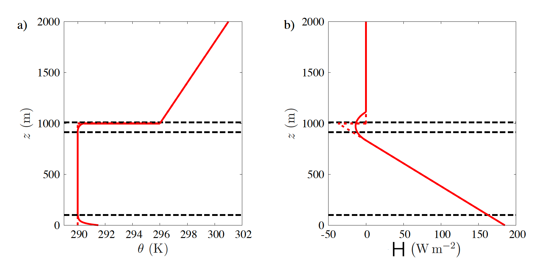
Fig. 20.6 Boundary layer profiles of potential temperature a and sensible heat flux b at 12 UTC. The dashed lines denote the idealized profiles.

The profiles are drawn in Fig. 20.6. From bottom to top, the layers are:

• the surface layer

• the mixed layer

• the entrainment zone

• the free troposphere

b) If \(h\) is 1000 m at 12 UTC, what is the boundary layer growth rate and the temperature change per hour in the CBL?

Hint

Assume (like in question 4b) that

\[ \overline{w'\theta'(h)}~=~-\beta \overline{w'\theta'(0)}, \]

where \(\beta\) is 0.2.

Answer

\[\begin{split} \afg{h}{t} &= 0.2 \frac{\overline{w'\theta'}(0)}{\Delta\theta}\\ \overline{w'\theta'}(0) &= 0.15\rm\,K\,m\,s^{-1}\\ \Delta\theta &= 6\rm\,K \end{split}\]

Therefore, \(\afg{h}{t} = 0.005\rm\,m\,s^{-1} = 18\,m\,hr^{-1}\)

\[\begin{split} \afg{\left<{\overline{\theta}}\right>}{t} &=\frac{\overline{w'\theta'}(0)-\overline{w'\theta'}(h)}{h} \\ &= \frac{\left(1+\beta\right)\overline{w'\theta'}(0)}{h}\\ h&= 1000\rm\,m \end{split}\]

Because of this, \(\afg{\left<{\overline{\theta}}\right>}{t} = 1.8\ \cdot 10^{-4}\rm\,K\,s^{-1}=0.65\,K\,hr^{-1}\).

c) Calculate the convective velocity at the same time and estimate how long it takes a parcel to travel from the surface to the top of the atmospheric boundary layer

Hint

The convective velocity is w*, which you derived in question 3a

Answer

The convective velocity is defined by

\[ w_*=\sqrt[3]{\frac{g}{\theta_v}\,\overline{w'\theta_v'}\,h} \]

In this definition, the buoyancy term of the TKE, \(\frac{g}{\theta_v}\,\overline{w'\theta_v'}\), is incorporated. In this case, no moisture is considered, so \(\overline{w'\theta_v'}=\overline{w'\theta'}\). Substituting the known values results in \(w_* = 1.72\rm\,m\,s^{-1}\).

The time it takes for a parcel to travel from the surface to the top of the atmospheric boundary layer due to convection is

\[ T = \frac{h}{w_*} \]

This results in \(T = 582 s \approx 10\rm\,min\)

20.6.

The one-dimensional conservation equation for heat reads:

\[ \pafg{\overline{\theta}}{t}~=~-~\pafg{\overline{w'\theta'}}{z} \]

a) Discuss which terms have been neglected from total conservation equation for heat to come to this equation

Hint

We derived the equation for the averaged potential temperature in week 2, exercise 4a.

\[ \underbrace{\gemafg{\theta}{t}}_{\rm Tendency} + \underbrace{\overline{u_j}\gemafg{\theta}{x_j}}_{\rm Advection} + \underbrace{\gemafg{u_j'\theta'}{x_j}}_{\rm Turbulent\ heat\ flux } = \underbrace{\nu_\theta\pafg{^2\overline{\theta}}{x_j^2}}_{\rm Molecular\ diffusion} - \underbrace{\frac{1}{\rho\,c_p}\gemafg{Q_j}{x_j}}_{\rm Radiation} - \underbrace{\frac{{ L_v}\,E}{\rho c_p}}_{\rm Latent\ heat\ release} \]

Answer

The total conservation equation for heat is

\[ \underbrace{\gemafg{\theta}{t}}_{\rm Tendency} + \underbrace{\overline{u_j}\gemafg{\theta}{x_j}}_{\rm Advection} + \underbrace{\gemafg{u_j'\theta'}{x_j}}_{\rm Turbulent\ heat\ flux } = \underbrace{\nu_\theta\pafg{^2\overline{\theta}}{x_j^2}}_{\rm Molecular\ diffusion} - \underbrace{\frac{1}{\rho\,c_p}\gemafg{Q_j}{x_j}}_{\rm Radiation} - \underbrace{\frac{{ L_v}\,E}{\rho c_p}}_{\rm Latent\ heat\ release} \]

The neglected terms are:

• advection: No advection is present. This automatically follows from using the assumption of horizontal homogeneity and the absence of subsidence.

• horizontal turbulent heat flux: Due to horizontal homogeneity, it is assumed that the horizontal turbulent heat flux is equal for all \(x\) and \(y\), causing the terms with \(i\) equal to 1 or 2 to vanish.

• diffusion: The impact of dissipation is relatively small under daytime (convective) conditions.

• radiation: The impact of radiation is relatively small under these conditions as well.

• latent heat release: In the case of clear skies, there is no condensation/evaporation.

b) Explain the mathematical steps and definitions to derive the mixed-layer equation for the bulk potential temperature that reads:

\[ \afg{ {\left< \overline{\theta}\right>}}{t}~=~\frac{\overline{w'\theta'(0)}-\overline{w'\theta'(h)}}{h}. \]

Answer

To get to the mixed-layer equations, the conservation equation has to be integrated with height over the whole boundary layer.

(20.2)\[ \int_{z_0}^h \! \pafg{\overline{\theta}}{t} \, dz = - \int_{z_0}^h \! \pafg{}{z}(\overline{w'\theta'}) dz \]

Integrating the right-hand-side of equation (20.2), we find:

(20.3)\[ - \int_{z_0}^h \! \pafg{}{z}(\overline{w'\theta'}) dz = \overline{w'\theta'}(z_0) - \overline{w'\theta'}(h) \]

Since one of the limits of the integration (\(h\)) is changing on time, we have to use of the Leibniz rule to solve the left-hand-side of integral (20.2):

For an arbitrary scalar, \(\psi\), and limits a and b, the Leibniz rule is:

(20.4)\[ \afg{}{t} \int_a^b \! \psi \, \mathrm{d}z = \int_a^b \! \pafg{\psi}{t} \, \mathrm{d}z - \psi(a) \afg{a}{t} + \psi(b) \afg{b}{t}. \]

We substitute \( \psi = \theta \) in Equation (20.4) and use the limits \(z_0\) and h. This gives:

\[ \afg{}{t} \underbrace{ \int_{z_0}^h \! \overline\theta \, dz}_{\left< \theta \right> h} =~ \int_{z_0}^h \!\pafg{\overline\theta }{t} \, dz- \underbrace{\overline\theta (z_0) \pafg{z_0}{t}}_{=0} + \overline\theta (h) \pafg{h}{t} \]

We reorganise this equation to find:

\[\begin{split} \int_{z_0}^h \! \pafg{\overline\theta}{t} \, dz &= \afg{}{t}[\left< \theta \right> h] - \overline\theta(h) \afg{h}{t}\\ &= h \afg{\left< \theta \right>}{t} + \left< \theta \right> \afg{h}{t} - \overline\theta(h) \afg{h}{t}\\ &= h \afg{\left< \theta \right>}{t} + \afg{h}{t} \underbrace{[\left< \theta \right>-\overline\theta(h)]}_{0} \end{split}\]

Throughout the mixed layer, \(\theta\) is homogeneous, so the second term cancels, resulting in:

(20.5)\[ \int_{z_0}^h \! \pafg{\overline{\theta}}{t} \, dz = h \afg{\left< \theta \right>}{t} \]

Finally, substitution of (20.5) and (20.3) on the original equation (20.2) results in:

\[ h \afg{\left< \theta \right>}{t} = \overline{w'\theta'}(z_0) - \overline{w'\theta'}(h) \]

or, alternatively:

(20.6)\[ \afg{\left< \theta \right>}{t} = \frac{1}{h}[ \overline{w'\theta'}(z_0) - \overline{w'\theta'}(h)] \]

c) Discuss the additional equations that we need to include the impact of the entrainment flux on the boundary layer growth.

Answer

The entrainment flux has to be related to the boundary layer growth rate:

\[\begin{split} \overline{w'\theta'}(h) &= - w_e \,\Delta\theta\\ &= - \afg{h}t \,\Delta\theta \end{split}\]

In this equation \(w_e\) is the entrainment velocity in m s\(^{-1}\) and \(\Delta\theta\) is the potential temperature jump at the inversion. In order to evaluate this equation, the time evolution of \(\Delta\theta\) has to be known. This is given by:

\[ \afg{\Delta\theta}{t} = \gamma_{\theta}\afg{h}{t}- \afg{\left<\overline{\theta}\right>}{t} \]

In the end, the system of governing equations is

\[\begin{split} \afg{\left<\overline{\theta}\right>}{t} &= \frac{\overline{w'\theta'}\left(z_0\right)-\overline{w'\theta'}\left(h\right)}{h}\\ \overline{w'\theta'}(h) &= - \afg{h}t \,\Delta\theta = -w_e \Delta\theta \\ \afg{\Delta\theta}{t} &= \gamma_{\theta}\afg{h}{t}- \afg{\left<\overline{\theta}\right>}{t} \end{split}\]

\(w_e\) is the entrainment velocity.